A typical HDD design consists of a spindle that holds flat circular disks, called platters, which hold the recorded data. The platters are made from a non-magnetic material, usually aluminum alloy, glass, or ceramic. They are coated with a shallow layer of magnetic material typically 10–20 nm in depth, with an outer layer of carbon for protection.
A strand of human DNA is 2.5 nanometers in diameter. Most proteins are about 10 nanometers wide, and a typical virus is about 100 nanometers wide. A bacterium is about 1000 nanometers. Human cells, such as red blood cells, are about 10,000 nanometers across. PM2.5 = matter that has a diameter of 2.5 micrometres or smaller.
In computer disk storage, a sector is a subdivision of a track on a magnetic disk or optical disc. For most disks, each sector stores a fixed amount of user-accessible data, traditionally 512 bytes for hard disk drives (HDDs) and 2048 bytes for CD-ROMs and DVD-ROMs. Newer HDDs and SSDs use 4096-byte (4 KiB) sectors, which are known as the Advanced Format (AF).
The sector is the minimum storage unit of a hard drive. Most disk partitioning schemes are designed to have files occupy an integral number of sectors regardless of the file’s actual size. Files that do not fill a whole sector will have the remainder of their last sector filled with zeroes.
Geometrically, the word sector means a portion of a disk between a center, two radii and a corresponding arc, which is shaped like a slice of a pie. Thus, the disk sector refers to the intersection of a track and geometrical sector.
In modern disk drives, each physical sector is made up of two basic parts, the sector header area (typically called “ID”) and the data area. The sector header contains information used by the drive and controller; this information includes sync bytes(that identifies the start of the sector, they merely indicate the start of the record.), address identification(sector number so the drive can know when it has found the start of a sector, and which sector it is), flaw flag and error detection and correction information. The header may also include an alternate address to be used if the data area is undependable. The address identification is used to ensure that the mechanics of the drive have positioned the read/write head over the correct location. The data area contains the sync bytes, user data and an error-correcting code (ECC) that is used to check and possibly correct errors that may have been introduced into the data.
还有一点要注意的是,上面Disk structures图里的实际上是老磁盘驱动器的样子,盘片是个圆,那么越靠外的磁道或扇区就比中心的越大,这意味着靠外的空间利用率就更差(因为逻辑上每个扇区都只能存512B或4KB)。现代的每个扇区在物理上也是一样大小,so they each store the same number of bits per unit areaper单位区域存的数据量就一样了(如下图)。
In modern hard drives, the amount of space between the head and rotating platter at normal operating speed is typically less than 5 nanometers… this gap is also referred to as the flying height.
磁头跟盘片距离5nm,参照上面的DNA是2.5nm。
读写技术
A modern HDD records data by magnetizing a thin film of ferromagnetic material on both sides of a disk. Sequential changes in the direction of magnetization represent binary data bits. The data is read from the disk by detecting the transitions in magnetization. User data is encoded using an encoding scheme, such as run-length limited encoding, which determines how the data is represented by the magnetic transitions.
Q = input(0) for i=1:size (input) if(Q = input(i)) 計數器+1 else output的前項=計數器的值, output的下一項=Q值, Q換成input(i),計數器值換成0 end end
output: 3A 1B 2C 1B 4C 2A(空格不存在)
寻道技术
before 1980s, CHS
Cylinder-Head-Sector,顾名思义,按柱面、磁头、扇区这个三维坐标定位扇区。
Head可以确定是disk中的哪一个盘片platter;Cylinder和Head可以共同确定是盘片上的哪一个磁道track;最后用Sector可以确定被定位的是哪一个数据块。This data block is an arc of (360/n) degrees, where n is the number of sectors in the track.
CHS addresses were exposed, instead of simple linear addresses (going from 0 to the total block count on disk - 1), because early hard drives didn’t come with an embedded disk controller, that would hide the physical layout. A separate generic controller card was used, so that the operating system had to know the exact physical “geometry” of the specific drive attached to the controller, to correctly address data blocks. The traditional limits were 512 bytes/sector × 63 sectors/track × 255 heads (tracks/cylinder) × 1024 cylinders, resulting in a limit of 8032.5 MiB for the total capacity of a disk.
As the geometry became more complicated (for example, with the introduction of zone bit recording) and drive sizes grew over time, the CHS addressing method became restrictive. Since the late 1980s, hard drives began shipping with an embedded disk controller that had good knowledge of the physical geometry. These logical CHS values would be translated by the controller, thus CHS addressing no longer corresponded to any physical attributes of the drive.
在 IBM PC 上,驱动软盘和硬盘的是 CPU 执行位于主板 BIOS (Basic Input/Output System) 中的程序,具体来说操作系统(比如DOS)和应用程序调用 INT 13H 中断,通过 AH=02H/03H 选择读/写操作,BIOS 在中断表中注册的 13H 中断处理程序执行在 CPU 上完成读写请求。调用 INT 13H 读写扇区的时候,CPU 先通过 INT 13H AH=0CH 控制硬盘的磁头臂旋转到特定柱面上,然后选定具体磁头,让磁头保持在磁道上读数据, 通过忙轮训的方式等待要读写的扇区旋转到磁头下方,从而读到所需扇区的数据。在 DOS 之后的操作系统, 比如早期的 Windows 和 Linux 和 BSD 能以覆盖中断程序入口表的方式提供升级版本的这些操作替代 BIOS 的程序。
after 1990s, LBA
Logical Block Addressing
where A is the LBA address, Nheads is the number of heads on the disk, Nsectors is the maximum number of sectors per track, and (c, h, s) is the CHS address.
For example, for geometry 1020 16 63 of a disk with 1028160 sectors, CHS 3 2 1 is LBA 3150 = ((3 × 16) + 2) × 63 + (1 – 1);
By the mid 1990s, hard drive interfaces replaced the CHS scheme with logical block addressing (LBA), but many tools for manipulating the master boot record (MBR) partition table still aligned partitions to cylinder boundaries; thus, artifacts of CHS addressing were still seen in partitioning software by the late 2000s.
1990年代中期,LBA取代了CHS定位,但很多操作master boot record (MBR)分区表的工具还在用CHS,所以知道2000年代末期还可以见到。
In the early 2010s, the disk size limitations imposed by MBR became problematic and the GUID Partition Table (GPT) was designed as a replacement; modern computers using UEFI firmware without MBR support no longer use any notions from CHS addressing.
橄榄球(Rugby)又称拉格比足球(Rugby football),源自其发源地拉格比公学(Rugby School,是位于英格兰中部沃里克郡拉格比镇上的一间男女兼收寄宿学校,也是英格兰最古老的公学之一,成立于1567年),香港简称为“榄球”,通常专指联合式橄榄球(Rugby Union football)或英式橄榄球,是一种使用椭圆形球进行奔跑推进得分的团体球类运动,是最早出现的橄榄球类运动。
美式橄榄球首先由哈佛大学学生以一种名叫“Ballown”的运动开始,这个运动的目的是要带着球跑过对手。在美国内战结束后美式橄榄球开始在大学中广泛流行。罗格斯学院和普林斯顿大学在1869年打了史上第一场大学美式橄榄球赛。这个运动最初跟英式足球相近,后来被人们改良至比较接近英式橄榄球。自1880年代起,被称为“美式橄榄球之父”的耶鲁大学教练沃尔特·坎普则把规则进一步改变,包括采用攻防线(line of scrimmage)和记档距离的比赛方式。1905年仍然有18位球员于比赛中受伤死亡。1906年又增加向前传球的规则,攻防线之间设置中立区(neutral zone),以及每队都要有至少6名球员于攻防线列阵,最重要的改革是首推将向前传球(抛传)合法化,使得真正意义上的美式橄榄球开始成形。
A football game is played between two teams of 11 players each. Teams may substitute any number of their players between downs. Individual players in a football game must be designated with a uniform number between 1 and 99.
除了offensive unit进攻球员和defensive unit防守球员还有特勤组,special teams unit。
Scoring
The touchdown (TD, 达阵6分), worth six points, is the most valuable scoring play in American football. A touchdown is scored when a live ball is advanced into, caught in, or recovered in the opposing team’s end zone.
The scoring team then attempts a try or conversion (附加得分), more commonly known as the point(s)-after-touchdown (PAT), which is a single scoring opportunity. A PAT is most commonly attempted from the two- or three-yard line, depending on the level of play. If a PAT is scored by a place kick or drop kick through the goal posts, it is worth one point, typically called the extra point. (踢进1分) If it is scored by what would normally be a touchdown it is worth two points, typically called the two-point conversion. (触地2分)
A field goal (FG, 射门3分), worth three points, is scored when the ball is place kicked (定点球, 一个人按着) or drop kicked (落地球, 球扔地上弹起来踢, rugby比较多而美式改尖后不好踢) through the uprights and over the crossbars of the defense’s goalposts.
After a PAT attempt or successful field goal, the scoring team must kick the ball off to the other team.
A safety (安全分,安防,自杀球2分) is scored when the ball carrier is tackled in his own end zone. Safeties are worth two points, which are awarded to the defense. In addition, the team that conceded the safety must kick the ball to the scoring team via a free kick.
Field and equipment
Football games are played on a rectangular field that measures 120 yards (110 m) long and $53\frac1{3}$ yards (48.8 m) wide.
end line底线, sideline边线, yard line分码线, hash marks码标, goal line得分线, end zone底线区/端区, goalposts/uprights球门柱.
Weighted pylons (达阵柱) are placed the sidelines on the inside corner of the intersections with the goal lines and end lines.
Duration and time stoppages
Football games last for a total of 60 minutes and are divided into two halves of 30 minutes and four quarters (节) of 15 minutes.
If a down is in progress when a quarter ends, play continues until the down is completed.
Games last longer than their defined length due to play stoppages—the average NFL game lasts slightly over three hours.
There are two main ways the offense can advance the ball: running and passing. In a typical play, the center (中锋) passes the ball backwards and between their legs to the quarterback (四分卫)in a process known as the snap (发球). The quarterback then either hands the ball off to a running back (跑卫), throws the ball, or runs with it. The play ends when the player with the ball is tackled or goes out-of-bounds or a pass hits the ground without a player having caught it. A forward pass can be legally attempted only if the passer is behind the line of scrimmage; only one forward pass can be attempted per down. As in rugby, players can also pass the ball backwards (向后传球) at any point during a play. In the NFL, a down also ends immediately if the runner’s helmet comes off.
The offense is given a series of four plays, known as downs. If the offense advances ten or more yards in the four downs, they are awarded a new set of four downs. (进攻有四档, 须推进>=10 yards)If they fail to advance ten yards, possession of the football is turned over to the defense. (turnover) In most situations, if the offense reaches their fourth down they will punt (弃踢, 方法是进攻队员(特勤组)把球扔下并在球落地之前将其踢向远处。通常进攻一方如果在前三档都未能成功前进十码,而该处位置又超过可以射门的距离,为免在攻守交换后让对方有机会可以在该处开始进攻,便会在第四档时使用弃踢大脚解围。) the ball to the other team, which forces them to begin their drive from farther down the field; if they are in field goal range (射门范围), they might attempt to score a field goal instead.
down (档, 即被对方拦截放倒一次) The offense must advance at least ten yards in four downs or plays; if they fail, they turn over the football to the defense, but if they succeed, they are given a new set of four downs to continue the drive.
There are two categories of kicks in football: scrimmage kicks, which can be executed by the offensive team on any down from behind or on the line of scrimmage (攻防线), and free kicks. The free kicks are the kickoff (开球。On a kickoff, the ball is placed at the 35-yard line; On a safety kick, the kicking team kicks the ball from their own 20-yard line.), which starts the first and third quarters and overtime and follows a try attempt or a successful field goal; the safety kick follows a safety (安防之后的安防踢不能用球座(tee), 需要扶球手, 也可以选safety punt).
They (after safety) can punt, drop kick or place kick the ball, but a tee (球座) may not be used in professional play. Any member of the receiving team may catch or advance the ball. The ball may be recovered by the kicking team once it has gone at least ten yards and has touched the ground or has been touched by any member of the receiving team.
The three types of scrimmage kicks are place kicks, drop kicks, and punts. Only place kicks and drop kicks can score points. The place kick is the standard method used to score points, because the pointy shape of the football makes it difficult to reliably drop kick. Once the ball has been kicked from a scrimmage kick, it can be advanced by the kicking team only if it is caught or recovered behind the line of scrimmage. If it is touched or recovered by the kicking team beyond this line, it becomes dead at the spot where it was touched. The kicking team is prohibited from interfering with the receiver’s opportunity to catch the ball. The receiving team has the option of signaling for a fair catch, which prohibits the defense from blocking into or tackling the receiver. The play ends as soon as the ball is caught and the ball may not be advanced.
Officials and fouls
裁判们,The back judge, The head linesman/down judge, The side judge, The line judge, The field judge, The center judge.
场上人数过多(Too many men on the field):任何一方在发球时超过十一人在场上均会被罚,后退五码。(注意:任何一方在交锋上少于十人都是合法;在2007年季赛中华盛顿红皮队为了纪念在屋中被劫杀的后卫尚•泰勒(Sean Taylor),特意在他死后的那周作客布法罗比尔队的比赛上,防守以十人列阵。)
A compressed package tarball is typically smaller than the compressed tarball containing the source code for the application.
Packages do not require compilation time. For large applications, such as Firefox, KDE Plasma, or GNOME, this can be important on a slow system.
Packages do not require any understanding of the process involved in compiling software on FreeBSD.
Port Benefits
Packages are normally compiled with conservative options because they have to run on the maximum number of systems. By compiling from the port, one can change the compilation options.
Some applications have compile-time options relating to which features are installed. For example, NGINX® can be configured with a wide variety of different built-in options.
In some cases, multiple packages will exist for the same application to specify certain settings. For example, NGINX® is available as a nginx package and a nginx-lite package, depending on whether or not Xorg is installed. Creating multiple packages rapidly becomes impossible if an application has more than one or two different compile-time options.
The licensing conditions of some software forbid binary distribution. Such software must be distributed as source code which must be compiled by the end-user.
Some people do not trust binary distributions or prefer to read through source code in order to look for potential problems.
Source code is needed in order to apply custom patches.
ports安装软件的基本流程, cd /usr/ports/net/wireshark 到需要安装的软件的源代码路径, make install clean 一步完成 make、 make install 和 make clean 这三个分开的步骤的工作。 ports使用fetch(1)下载,设置代理也是对fetch配置环境变量,详细的fetch(3)。 顺带一提,FreeBSD里下载某个文件也是fetch url即可。
Yeah, “make deinstall” uses the information in the port Makefile and pkg-plist to see what to remove. If the version in the Makefile is not identical to the installed version, files can be left behind or accidentally deleted.
“pkg_delete” uses the information in /var/db/pkg, which corresponds to what’s actually on the disk.
“make deinstall” and “make reinstall” should really only be used for testing. “pkg_delete” and “make install” are better, more reliable tools. phoenix也提到除了测试时尽量不要用。
root@nas:/ # geom part list root@nas:/ # gpart create -s GPT ada0 The partition scheme is created, andthen a single partition is added. To improve performance on newer disks with larger hardware block sizes, the partition is aligned to one megabyte boundaries: root@nas:/ # gpart add -t freebsd-ufs -a 1M ada0 Depending on use, several smaller partitions may be desired. See gpart(8) for options to create partitions smaller than a whole disk. The disk partition information can be viewed with gpart show: root@nas:/home/V2beach/Desktop # gpart show ada0 => 40976773088 ada0 GPT (466G) 402008 - free - (1.0M) 20489767710721 freebsd-ufs (466G) 9767731208 - free - (4.0K) A file system is created in the new partition on the new disk: root@nas:/ # newfs -U /dev/ada0p1 /dev/ada0p1: 476939.0MB (976771072 sectors) block size 32768, fragment size 4096 using763 cylinder groups of625.22MB, 20007 blks, 80128 inodes. with soft updates super-block backups (for fsck_ffs -b #) at: 192, 1280640, 2561088, 3841536, 5121984, 6402432, 7682880, 8963328, 10243776, ... An empty directory is created as a mountpoint, a location for mounting the new disk in the original disk’s file system: root@nas:/ # mkdir /newdisk root@nas:/ # mount /dev/ada0p1 /newdisk root@nas:/ # chmod 777 /newdisk
DLNA(Digital Living Network Alliance 数字生活联盟),根据spirespark文档,协议集包括以下部分,
Functional Components
Technology Ingredients
Connectivity
Ethernet, 802.11 (including Wi-Fi Direct), MoCA, HD-PLC, HomePlug-AV, HPNA and Bluetooth
Networking
IPv4 and IPV6 Suite
Device Discovery and Control
UPnP* Device Architecture
Media Management and Control
UPnP AV, EnergyManagement, DeviceManagement, and Printer
Media Formats
Required and Optional Format Profiles
Media Transport
HTTP (Mandatory) , HTTP Adaptive Delivery (DASH) and RTP
Remote User Interfaces
CEA-2014-A , HTML5
Device Profiles
CVP-NA-1, CVP-EU-1, CVP-2
这么看不太直观,对比OSI或者TCP/IP模型就能看的比较清楚, 数据链路层802系列协议,网络层IP协议,传输层的TCP和UDP分别支持下面图上的应用层HTTP/UPnP协议。 其中核心是UPnP(Universal Plug and Play 通用即插即用),实现了DLNA的设备发现、控制等基本功能。
UPnP assumes the network runs IP and then leverages HTTP, on top of IP, in order to provide device/service description, actions, data transfer and event notification. Device search requests and advertisements are supported by running HTTP on top of UDP (port 1900) using multicast (known as HTTPMU). Responses to search requests are also sent over UDP, but are instead sent using unicast (known as HTTPU). UPnP uses UDP due to its lower overhead in not requiring confirmation of received data and retransmission of corrupt packets. UPnP uses UDP port 1900 and all used TCP ports are derived from the SSDP alive and response messages.
UPnP假定网络运行着Internet Protocol并且利用IP之上的HTTP,提供设备或服务的描述、活动、数据交换和事件通知。设备发现请求由HTTPMU实现(UDP1900端口上的广播HTTP请求);响应由HTTPU(Hypertext Transfer or Transport Protocol over UDP)实现,是单播的,也用UDP。 UPnP用UDP是因为开销较低(不需要确认收到数据且不需要重传损坏的包)。UPnP用UDP1900端口,所有用到的TCP端口都源于SSDP活跃的响应消息。
Conceptually, UPnP extends plug and play—a technology for dynamically attaching devices directly to a computer—to zero-configuration networking for residential and SOHO wireless networks.
UPnP的Control Points(CPs控制点)使用UPnP控制Controlled Devices(CDs被控制设备),Dynamic Host Configuration Protocol (DHCP) and Domain Name System (DNS) servers are optional and are only used if they are available on the network. DHCP和DNS服务器都是可选的。
UPnP的作用过程如下,
Addressing The foundation for UPnP networking is IP addressing. Each device must implement a DHCP client and search for a DHCP server when the device is first connected to the network. If no DHCP server is available, the device must assign itself an address. The process by which a UPnP device assigns itself an address is known within the UPnP Device Architecture as AutoIP. If during the DHCP transaction, the device obtains a domain name, for example, through a DNS server or via DNS forwarding, the device should use that name in subsequent network operations; otherwise, the device should use its IP address.
Discovery Once a device has established an IP address, the next step in UPnP networking is discovery. The UPnP discovery protocol is known as the Simple Service Discovery Protocol (SSDP). When a device is added to the network, SSDP allows that device to advertise its services to control points on the network. This is achieved by sending SSDP alive messages. When a control point is added to the network, SSDP allows that control point to actively search for devices of interest on the network or listen passively to the SSDP alive messages of devices. The fundamental exchange is a discovery message containing a few essential specifics about the device or one of its services, for example, its type, identifier, and a pointer (network location) to more detailed information.
Description After a control point has discovered a device, the control point still knows very little about the device. For the control point to learn more about the device and its capabilities, or to interact with the device, the control point must retrieve the device’s description from the location (URL) provided by the device in the discovery message. The UPnP Device Description is expressed in XML and includes vendor-specific manufacturer information like the model name and number, serial number, manufacturer name, (presentation) URLs to vendor-specific web sites, etc. The description also includes a list of any embedded services. For each service, the Device Description document lists the URLs for control, eventing and service description. Each service description includes a list of the commands, or actions, to which the service responds, and parameters, or arguments, for each action; the description for a service also includes a list of variables; these variables model the state of the service at run time, and are described in terms of their data type, range, and event characteristics.
Control Having retrieved a description of the device, the control point can send actions to a device’s service. To do this, a control point sends a suitable control message to the control URL for the service (provided in the device description). Control messages are also expressed in XML using the Simple Object Access Protocol (SOAP). Much like function calls, the service returns any action-specific values in response to the control message.
Event Notification Another capability of UPnP networking is event notification, or eventing. The event notification protocol defined in the UPnP Device Architecture is known as General Event Notification Architecture (GENA). A UPnP description for a service includes a list of actions the service responds to and a list of variables that model the state of the service at run time. The service publishes updates when these variables change, and a control point may subscribe to receive this information. The service publishes updates by sending event messages. Event messages contain the names of one or more state variables and the current value of those variables. These messages are also expressed in XML.
Presentation The final step in UPnP networking is presentation. If a device has a URL for presentation, then the control point can retrieve a page from this URL, load the page into a web browser, and depending on the capabilities of the page, allow a user to control the device and/or view device status.
NAT traversal One solution for NAT traversal, called the Internet Gateway Device Protocol (IGD Protocol), is implemented via UPnP. Many routers and firewalls expose themselves as Internet Gateway Devices, allowing any local UPnP control point to perform a variety of actions, including retrieving the external IP address of the device, enumerating existing port mappings, and adding or removing port mappings. By adding a port mapping, a UPnP controller behind the IGD can enable traversal of the IGD from an external address to an internal client.
root@nas:/ # pkg install samba
root@nas:/ # vim /usr/local/etc/smb4.conf
/usr/local/etc/smb4.conf
[global]
workgroup          = WORKGROUP
netbios name       = freebsd-test
server string      = samba
security           = user
wins support       = yes
passdb backend     = tdbsam

# Following is the data directory you want to share.

[SMBshare]
  path = /newdisk
  valid users = V2beach
  public = no
  writable  = yes
  browsable  = yes
  read only = no
  guest ok = no
  create mask = 0755
  directory mask = 0755
root@nas:/home/V2beach/Desktop # pdbedit -a -u V2beach new password: retype new password: Unix username: V2beach NT username: Account Flags: [U ] User SID: S-1-5-21-1459039941-1455980450-4236412286-1000 Primary Group SID: S-1-5-21-1459039941-1455980450-4236412286-513 Full Name: Hulk Leo Home Directory: \\FREEBSD-TEST\v2beach HomeDir Drive: Logon Script: Profile Path: \\FREEBSD-TEST\v2beach\profile Domain: FREEBSD-TEST Account desc: Workstations: Munged dial: Logon time: 0 Logoff time: Wed, 06 Feb 203623:06:39 CST Kickoff time: Wed, 06 Feb 203623:06:39 CST Password last set: Mon, 25 Sep 202301:34:38 CST Password can change: Mon, 25 Sep 202301:34:38 CST Password must change: never Last bad password : 0 Bad password count : 0 Logon hours : FFFFFFFFFFFFFFFFFFFFFFFFFFFFFFFFFFFFFFFFFF root@nas:/home/V2beach/Desktop #
root@nas:/ #  vim /etc/rc.conf
samba_enable="YES "
samba_server_enable="YES"
root@nas:/ # service samba_server start
root@nas:/ # service samba_server status
client
windows
开服务之后在文件窗口输\\192.168.x.x(NAS的IP地址)\SMBshare。
macos
finder里connect to server,连smb://192.168.x.x/SMBshare。
Server Message Block (SMB) enables file sharing, printer sharing, network browsing, and inter-process communication (through named pipes) over a computer network. SMB serves as the basis for Microsoft’s Distributed File System implementation. SMB relies on the TCP and IP protocols for transport. This combination allows file sharing over complex, interconnected networks, including the public Internet. The SMB server component uses TCP port 445. SMB originally operated on NetBIOS over IEEE 802.2 - NetBIOS Frames or NBF - and over IPX/SPX, and later on NetBIOS over TCP/IP (NetBT), but Microsoft has since deprecated these protocols. On NetBT, the server component uses three TCP or UDP ports: 137 (NETBIOS Name Service), 138 (NETBIOS Datagram Service), and 139 (NETBIOS Session Service).
root@nas:/ # setenv D /usr/jail/vim-adventure root@nas:/ # mkdir -p $D root@nas:/ # cd /usr/src root@nas:/ # make buildworld -------------------------------------------------------------- >>> World build completed on Wed Sep 2714:21:17 CST 2023 >>> World built in14389 seconds, ncpu: 4 -------------------------------------------------------------- root@nas:/ # make installworld DESTDIR=$D root@nas:/ # make distribution DESTDIR=$D root@nas:/ # mount -t devfs devfs $D/dev
或者直接下载base,
fetch https://download.freebsd.org/ftp/releases/amd64/amd64/13.2-RELEASE/base.txz -o /usr/local/jails/media/13.2-RELEASE-base.txz
tar -xvf /usr/local/jails/media/13.2-RELEASE-base.txz -C /usr/jail/vim-adventure/
root@nas:/usr/ports/lang/mono # make install clean (太慢) root@nas:/usr/ports/lang/mono # make all-depends-list (太多) root@nas:/ # pkg install mono ffmpeg mediainfo root@nas:/ # pkg install python The following 2 package(s) will be affected (of0 checked): New packages to be INSTALLED: python: 3.9_3,2 python3: 3_3 Number of packages to be installed: 2 2 KiB to be downloaded. root@nas:/ # pkg install py39-pip root@nas:/ # pip install --no-build-isolation Differential --proxy http://127.0.0.1:8001
In mathematics parity can refer to the evenness or oddness of an integer, which, when written in its binary form, can be determined just by examining only its least significant bit.
The parity bit ensures that the total number of 1-bits in the string is even or odd. Accordingly, there are two variants of parity bits: even parity bit and odd parity bit. In the case of even parity, for a given set of bits, the bits whose value is 1 are counted. In the case of even parity, for a given set of bits, the bits whose value is 1 are counted. If that count is odd, the parity bit value is set to 1, making the total count of occurrences of 1s in the whole set (including the parity bit) an even number. If the count of 1s in a given set of bits is already even, the parity bit’s value is 0. In the case of odd parity, the coding is reversed. Even parity is a special case of a cyclic redundancy check (CRC), where the 1-bit CRC is generated by the polynomial x+1.
奇偶校验位确保整个二进制数的“1”有偶数个或者奇数个。因此有两种变体:偶数校验位和奇数校验位。偶数校验位是如果二进制数原本有奇数个1,那就在LSB上补一个1让整个二进制数的1有偶数个,如果原本就有偶数个1,那只需要补一个0,保持偶数个;奇数校验位反之。 偶数校验位是一种循环冗余校验CRC,一个特例,通过多项式 x + 1 得到1位CRC。
For example, suppose two drives in a three-drive RAID 5 array contained the following data:
In electronics, transcoding data with parity can be very efficient, as XOR gates output what is equivalent to a check bit that creates an even parity, and XOR logic design easily scales to any number of inputs. XOR and AND structures comprise the bulk of most integrated circuitry.
Y = A’ · B + A · B’ = A XOR B XOR (/ˌɛks ˈɔːr/, /ˌɛks ˈɔː/, /ˈksɔːr/ or /ˈksɔː/), EOR, EXOR, $\oplus$, $\nleftrightarrow$, $\not \equiv $. Exclusive or.
上面提到过,偶数校验位实际是通过多项式 x + 1 得到1位CRC的循环冗余校验,那在探索CRC之前必须学一下GF有限域。 在学习的时候遇到了一些困难,首先是定义和性质,看得我云里雾里,分别看了维基百科、知乎和这篇文章的翻译出处Channel Codes: Classical and Modern(之后找个地方上传一下这些资源)之后,仍然没有搞清楚定义和性质的推导,不过好在对有限域的运算理解了一些,这已经足够大概理解CRC了。
以下定义将直接摘抄自Channel Codes: Classical and Modern,这本书是美籍华人Adjunct Professor林舒和William E. Ryan的著作(2009年)。
Field
一个基本概念——
Definition 2.2. Let S be a set with a binary operation ∗. The operation is said to be commutative if, given any two elements, a and b, in S, the following equality holds: a∗b = b∗a. (2.2) We also say that ∗ satisfies the commutative law, if (2.2) holds.
2.3 Fields In this section, we introduce an algebraic system with two binary operations, called a field. Fields with finite numbers of elements, called finite fields, play an important role in developing algebraic coding theory and constructing error-correction codes that can be efficiently encoded and decoded. Well-known and widely used error-correction codes in communication and storage systems based on finite fields are BCH (Bose–Chaudhuri–Hocquenghem) codes and RS (Reed–Solomon) codes, which were introduced at the very beginning of the 1960s. Most recently, finite fields have successfully been used for constructing low-density parity-check (LDPC) codes that perform close to the Shannon limit with iterative decoding.
在信道编码的2.3节中,在介绍完2.1集合和二元运算(Sets and Binary Operations)、2.2群(Groups)之后,开始讲解有两个二元运算的代数系统——域。包含有限元素的域叫做有限域(galois),有限域在代数编码理论的发展中、在构建能高效编解码的错误校正编码中扮演了重要角色。在通信和存储系统中,基于有限域的广为人知的错误校正码有BCH码、RS码,都是在六十年代早期被发明的。最近,有限域被成功地用在构建通过迭代解码、性能接近香农极限的低密度奇偶检测(LDPC)码上。
2.3.1 Definitions and Basic Concepts Definition 2.8. Let F be a set of elements on which two binary operations, called addition ‘‘+’’ and multiplication ‘‘·,’’ are defined. F is a field under these two operations, addition and multiplication, if the following conditions (or axioms) are satisfied.
F is a commutative group under addition +. The identity element with respect to addition + is called the zero element (or additive identity) of F and is denoted by 0.
The set F\\{0} of nonzero elements of F forms a commutative group under multiplication ·. The identity element with respect to multiplication · is called the unit element (or multiplicative identity) of F and is denoted by 1.
For any three elements a, b, and c in F, $a·(b+c) = a·b+a·c$ The equality is called the distributive law, i.e., multiplication is distributive over addition.
集合F\\{0}(the set that contains the elements in X but not in Y is called the difference between X and Y and is denoted by X\\Y)即没有0元素的F构成了乘法的交换群。乘法相关的恒等元叫做单位元或乘法单位元,用1表示。
From the definition, we see that a field consists of two groups with respect to two operations, addition and multiplication. The group with respect to addition is called the additive group of the field, and the group with respect to multiplication is called the multiplicative group of the field. Since each group must contain an identity element, a field must contain at least two elements. Later, we will show that a field with two elements does exist. In a field, the additive inverse of an element a is denoted by ‘‘−a,’’ and the multiplicative inverse of a is denoted by ‘‘a−1,’’ provided that a ̸= 0. From the additive and multiplicative inverses of ele- ments of a field, two other operations, namely subtraction ‘‘−’’ and division ‘‘÷,’’ can be defined. A field is simply an algebraic system in which we can perform addition, subtraction, multiplication, and division without leaving the field.
根据定义,可以发现一个域包含两个关于二元操作的群,加法和乘法。关于加法的叫做域的加法群,关于乘法的叫域的乘法群。因为每个群必须包含一个恒等元(单位元),所以一个域至少包含两个元素{0, 1}。之后会证明两个元素的域确实存在。在域中,加法的a反过来记作“-a”,乘法的a反过来记作“a-1”(a均不等于0),从这两个相反(逆运算)可以得到subtraction ‘‘−’’ 减和division ‘‘÷” 除操作。$a − b \triangleq a + (−b)$,很明显a-a=0;$a ÷ b \triangleq a · (b−1)$,很明显a÷a=1。 域就是可以在域中的任意元素上做加减乘除运算,结果仍在域内的代数系统。
Definition 2.9. The number of elements in a field is called the order of the field. A field with finite order is called a finite field. Definition 2.10. Let F be a field. A subset K of F that is itself a field under the operations of F is called a subfield of F. In this context, F is called an extension field of K. If K ̸= F, we say that K is a proper subfield of F. A field containing no proper subfields is called a prime field. Definition 2.11. Let F be a field and 1 be its unit element (or multiplicative identity). The characteristic of F is defined as the smallest positive integer λ such that $\sum_{i=1}^\lambda 1=\underbrace{1+1+\cdots+1}_\lambda=0$ where the summation represents repeated applications of addition + of the field. If no such λ exists, F is said to have zero characteristic, i.e., λ = 0, and F is an infinite field. Theorem 2.4. The characteristic λ of a finite field is a prime.
2.3.2 Finite Fields The rational-, real- and complex-number fields are infinite fields. In error-control coding, both theory and practice, we mainly use finite fields. Let p be a prime number. In Section 2.2.2, we have shown that the set of inte- gers, {0, 1, . . ., p − 1}, forms a commutative group under modulo-p addition $\boxplus$. We have also shown that the set of nonzero elements, {1, 2, . . ., p − 1}, forms a commutative group under modulo-p multiplication $\boxdot$. Following the definitions of modulo-p addition and multiplication and the fact that real-number multiplication is distributive over real number addition, we can readily show that the modulo-p multiplication is distributive over modulo-p addition. Therefore, the set of integers, {0, 1, . . ., p − 1}, forms a finite field GF(p) of order p under modulo-p addition and multiplication, where 0 and 1 are the zero and unit elements of the field, respectively. The following sums of the unit element 1 give all the elements of the field: $1, \quad \sum_{i=1}^2 1=2, \quad \sum_{i=1}^3 1=1 \boxplus 1 \boxplus 1=3, \quad \ldots, \quad \sum_{i=1}^{p-1} 1=p-1, \quad \sum_{i=1}^p 1=0$ Since p is the smallest positive integer such that $\sum_{i=1}^p 1=0$, the characteristic of the field is p. The field contains no proper subfield and hence is a prime field.
Example 2.8. Consider the special case for which p = 2. For this case, the set {0, 1} under modulo-2 addition and multiplication as given by Tables 2.6 and 2.7 forms a field of two elements, denoted by GF(2). Note that {1} forms the multiplicative group of GF(2), a group with only one element. The two elements of GF(2) are simply the additive and multiplicative identities of the two groups of GF(2). The additive inverses of 0 and 1 are themselves. This implies that 1 − 1 = 1 + 1. Hence, over GF(2), subtraction and addition are the same. The multiplicative inverse of 1 is itself. GF(2) is commonly called a binary field, the simplest finite field. GF(2) plays an important role in coding theory and is most commonly used as the alphabet of code symbols for error-correction codes.
We have shown that, for every prime number p, there exists a prime field GF(p). For any positive integer m, it is possible to construct a Galois field $GF(p^m)$ with $p^m$ elements based on the prime field GF(p) and a root of a special irreducible polynomial with coefficients from GF(p). This will be shown in a later section. The Galois field $GF(p^m)$ contains GF(p) as a subfield and is an extension field of GF(p). A very important feature of a finite field is that its order must be a power of a prime. That is to say that the order of any finite field is a power of a prime.
Definition 2.12. Let a be a nonzero element of a finite field GF(q). The smallest positive integer n such that $a^n = 1$ is called the order of the nonzero field element a. Theorem 2.5. Let a be a nonzero element of order n in a finite field GF(q). Then the powers of a, $a^n=1, a, a^2, \ldots, a^{n-1}$ form a cyclic subgroup of the multiplicative group of GF(q). Theorem 2.6. Let a be a nonzero element of a finite field GF(q). Then $a^{q−1} = 1$. Theorem 2.7. Let n be the order of a nonzero element a in GF(q). Then n divides q − 1. Definition 2.13. A nonzero element a of a finite field GF(q) is called a primitive element if its order is q − 1. That is, $a^{q−1} = 1,a,a2, …,a^{q−2}$ form all the nonzero elements of GF(q).
定义,设a是有限域GF(q)的非零元素,能使$a^n = 1$的最小的正整数n叫做非零域元素a的阶。 定理,设a是阶为n的有限域GF(q)上的非零元素,a的幂构成了GF(q)乘法群的一个循环子群。 定理,设a是有限域GF(q)的非零元素,则$a^{q−1} = 1$。 定律,设n是有限域GF(q)上非零元素a的阶,那么n能整除q-1即(q-1) mod n = 0。比如GF(5)上2的阶是4,$2^4=16\ mod\ 5 = 1$,4 mod 4 = 0。证明都在书上,我就不贴了。 定义,有限域GF(q)的非零元素a如果阶是q - 1则被称作本原元。即$a^{q−1} = 1,a,a2, …,a^{q−2}$构成了GF(q)的所有非零元素。
Polynomials over Finite Fields
2.5 Polynomials over Finite Fields In this section, we consider polynomials with coefficients from a finite field GF(q), which are used in error-control coding theory. A polynomial with one variable (or indeterminate) X over GF(q) is an expression of the following form: $a(X) = a_0 + a_1X + …, a_nX^{n}$ where n is a non-negative integer and the coefficients $a_i$, 0 ≤ i ≤ n, are elements of GF(q). The degree of a polynomial is defined as the largest power of X with a nonzero coefficient. For the polynomial a(X) above, if $a_n \neq 0$, its degree is n; if $a_n = 0$, its degree is less than n. The degree of a polynomial $a(X) = a_0$ with only the constant term is zero. We use the notation deg(a(X)) to denote the degree of polynomial a(X). A polynomial is called monic if the coefficient of the highest power of X is 1 (the unit element of GF(q)). The polynomial whose coefficients are all equal to zero is called the zero polynomial and denoted by 0.
$a(X) \cdot b(X)=c_{0}+c_{1} X+\cdots+c_{k} X^{k}+\cdots+c_{n+m} X^{n+m}$ $c_{k}=\sum_{\substack{i+j=k, 0 \leq i \leq n, 0 \leq j \leq m}} a_{i} \cdot b_{j}$
we can readily verify that the polynomials over $\operatorname{GF}(q)$ satisfy the following conditions.
Associative laws. For any three polynomials $a(X), b(X)$, and $c(X)$ over $\mathrm{GF}(q)$,
Commutative laws. For any two polynomials $a(X)$ and $b(X)$ over $\operatorname{GF}(q)$,
Distributive law. For any three polynomials $a(X), b(X)$, and $c(X)$ over $\mathrm{GF}(q)$,
In algebra, the set of polynomials over $\operatorname{GF}(q)$ under polynomial addition and multiplication defined above is called a polynomial ring over $\mathrm{GF}(q)$.
Subtraction
Subtraction of $b(X)$ from $a(X)$ is carried out as follows:
where $a_{i}-b_{i}=a_{i}+\left(-b_{i}\right)$ is carried out in $\operatorname{GF}(q)$ and $-b_{i}$ is the additive inverse of $b_{i}$.
Division
Definition 2.19. A set $\mathcal{R}$ with two binary operations, called addition + and multiplication $\cdot$, is called a ring, if the following axioms are satisfied.
$\mathcal{R}$ is a commutative group with respect to + .
Multiplication “.” is associative, i.e., $(a \cdot b) \cdot c=a \cdot(b \cdot c)$ for all $a, b, c \in \mathcal{R}$.
The distributive laws hold: for $a, b, c \in \mathcal{R}, a \cdot(b+c)=a \cdot b+a \cdot c$ and $(b+c) \cdot a=b \cdot a+b \cdot a$.
The set of all polynomials over $\operatorname{GF}(q)$ defined above satisfies all three axioms of a ring. Therefore, it is a ring of polynomials. The set of all integers under real addition and multiplication is a ring. For any positive integer $m \geq 2$, the set $\mathcal{R}=$ $\{0,1, \ldots, m-1\}$ under modulo- $m$ addition and multiplication forms a ring (the proof is left as an exercise). In Section 2.3, it was shown that, if $m$ is a prime, $\mathcal{R}=$ $\{0,1, \ldots, m-1\}$ is a prime field under modulo- $m$ addition and multiplication.
Let $a(X)$ and $b(X)$ be two polynomials over $\operatorname{GF}(q)$. Suppose that $b(X)$ is not the zero polynomial, i.e., $b(X) \neq 0$. When $a(X)$ is divided by $b(X)$, we obtain a unique pair of polynomials over $\mathrm{GF}(q), q(X)$ and $r(X)$, such that
where $0 \leq \operatorname{deg}(r(X))<\operatorname{deg}(b(X))$ and the polynomials $q(X)$ and $r(X)$ are called the quotient and remainder, respectively. This is known as Euclid’s division algorithm. The quotient $q(x)$ and remainder $r(X)$ can be obtained by ordinary long division of polynomials. If $r(X)=0$, we say that $a(X)$ is divisible by $b(X)$ (or $b(X)$ divides $a(X))$.
$a(X)=q(X) \cdot b(X)+r(X)$其中$0 \leq \operatorname{deg}(r(X)),<\operatorname{deg}(b(X))$,多项式$q(X)$和$r(X)$分别被称为商和余,即欧几里得除法,$q(X)$和$r(X)$可以由多项式的长除算得。如果$r(X)$,我们就说$b(X)$整除$a(X)$,即$a(X)$ mod $b(X)$ = 0。 除法比较复杂所以演算一个书上的例子。
Example 2.13. Let $a(x)=3+4 X+X^{4}+2 X^{5}$ and $b(X)=1+3 X^{2}$. Suppose we divide $a(X)$ by $b(X)$. Using long division,
定理和性质就不再讨论了,理解CRC需要的知识现在都具备了。
Cyclic Redundancy Check
Introduction
A cyclic redundancy check (CRC) is an error-detecting code commonly used in digital networks and storage devices to detect accidental changes to digital data. Blocks of data entering these systems get a short check value attached, based on the remainder of a polynomial division of their contents. CRCs are so called because the check (data verification) value is a redundancy (it expands the message without adding information) and the algorithm is based on cyclic codes. CRCs are popular because they are simple to implement in binary hardware, easy to analyze mathematically, and particularly good at detecting common errors caused by noise in transmission channels. Because the check value has a fixed length, the function that generates it is occasionally used as a hash function.
Specification of a CRC code requires definition of a so-called generator polynomial. This polynomial becomes the divisor in a polynomial long division, which takes the message as the dividend and in which the quotient is discarded and the remainder becomes the result. The important caveat is that the polynomial coefficients are calculated according to the arithmetic of a finite field, so the addition operation can always be performed bitwise-parallel (there is no carry between digits). In practice, all commonly used CRCs employ the finite field of two elements, GF(2). The two elements are usually called 0 and 1, comfortably matching computer architecture.
CRCs are specifically designed to protect against common types of errors on communication channels, where they can provide quick and reasonable assurance of the integrity of messages delivered. However, they are not suitable for protecting against intentional alteration of data. an attacker can edit a message and recompute the CRC without the substitution being detected. unlike cryptographic hash functions, CRC is an easily reversible function, which makes it unsuitable for use in digital signatures.
Binary form:101  divided by  11
Decimal form:5  divided by  3

x**2+1
x+1

Divide operation:

Result is11
Remainder is0
Working is

 11
---
101
11
--
 11
 11
 --
  0
import struct import sys val1='1010' val2='110'
if (len(sys.argv)>1): val1=str(sys.argv[1])
if (len(sys.argv)>2): val2=str(sys.argv[2])
defshowpoly(a): str1 = "" nobits = len(a) for x in range (0,nobits-2): if (a[x] == '1'): if (len(str1)==0): str1 +="x**"+str(nobits-x-1) else: str1 +="+x**"+str(nobits-x-1) if (a[nobits-2] == '1'): if (len(str1)==0): str1 +="x" else: str1 +="+x"
if (a[nobits-1] == '1'): str1 +="+1" print(str1)
deftoList(x): l = [] for i in range (0,len(x)): l.append(int(x[i])) return (l)
deftoString(x): str1 ="" for i in range (0,len(x)): str1+=str(x[i]) return (str1)
defdivide(val1,val2): a = toList(val1) b = toList(val2) working="" res="" while len(b) <= len(a) and a: if (a[0] == 1): del a[0] for j in range(len(b)-1): a[j] ^= b[j+1] if (len(a)>0): working +=toString(a) res+= "1" else: del a[0] working +=toString(a) res+="0" print("Result is\t",res) print("Remainder is\t",toString(a)) return
print("Binary form:\t",val1," divided by ",val2) print("Decimal form:\t",int(val1,2)," divided by ",int(val2,2)) print("")
To compute an n-bit binary CRC, line the bits representing the input in a row, and position the (n + 1)-bit pattern representing the CRC’s divisor (called a “polynomial”) underneath the left end of the row. In this example, we shall encode 14 bits of message with a 3-bit CRC, with a polynomial x^3 + x + 1. The polynomial is written in binary as the coefficients; a 3rd-degree polynomial has 4 coefficients (1x^3 + 0x^2 + 1x + 1). In this case, the coefficients are 1, 0, 1 and 1. The result of the calculation is 3 bits long, which is why it is called a 3-bit CRC. However, you need 4 bits to explicitly state the polynomial.
This is first padded with zeros corresponding to the bit length n of the CRC. This is done so that the resulting code word is in systematic form. Here is the first calculation for computing a 3-bit CRC:
11010011101100 000 <--- input right padded by 3 bits
1011               <--- divisor (4 bits) = x³ + x + 1
------------------
01100011101100 000 <--- result
The algorithm acts on the bits directly above the divisor in each step. The result for that iteration is the bitwise XOR of the polynomial divisor with the bits above it. The bits not above the divisor are simply copied directly below for that step. The divisor is then shifted right to align with the highest remaining 1 bit in the input, and the process is repeated until the divisor reaches the right-hand end of the input row. Here is the entire calculation:
11010011101100 000 <--- input right padded by 3 bits
1011               <--- divisor
01100011101100 000 <--- result (note the first four bits are the XOR with the divisor beneath, the rest of the bits are unchanged)
 1011              <--- divisor ...
00111011101100 000
  1011
00010111101100 000
   1011
00000001101100 000 <--- note that the divisor moves over to align with the next 1 in the dividend (since quotient for that step was zero)
       1011             (in other words, it doesn't necessarily move one bit per iteration)
00000000110100 000
        1011
00000000011000 000
         1011
00000000001110 000
          1011
00000000000101 000
           101 1
-----------------
00000000000000 100 <--- remainder (3 bits).  Division algorithm stops here as dividend is equal to zero.
Since the leftmost divisor bit zeroed every input bit it touched, when this process ends the only bits in the input row that can be nonzero are the n bits at the right-hand end of the row. These n bits are the remainder of the division step, and will also be the value of the CRC function (unless the chosen CRC specification calls for some postprocessing). The validity of a received message can easily be verified by performing the above calculation again, this time with the check value added instead of zeroes. The remainder should equal zero if there are no detectable errors.
約好出來吃飯的朋友因為復感染Coronavirus-19沒法一起慶生了,今天的計畫是,今天沒有計畫,不過反正中午燒烤、晚上燒烤,杭州的摩天輪在妳媽蕭山區36km,性價比比較高的獵鷹射擊在下沙20+km,但杭州樂園和獵鷹距離也有20+km… 說實話300~500人民幣在美國夠買上千發了吧,在國內只能射20發手槍+10發氣槍鉛彈。算了今天去西湖轉轉吧,約煜謙明天去打靶,今晚去夜店!健身放假一天,遊戲放假一天,英語放假一天。 說起來,昨天跟王阿姨打電話,聽到她說她身邊特別多的出國案例,也提到一個直到申請季沒考出托福,因為國內疫情關考場不得已去東南亞考試的案例,似乎是跟我很像的拖延,包括她女兒多倫多芝大回國實習的履歷,心裡咯噔一下。我是真的該全力考托考G了。 But anyway, I should enjoy my life, abstain from being that anxious anymore, everything is gonna be alright, that’s the most important thing I learned last year.
]]>
<p>祝自己生日快樂。:D</p>
Timeline of the British Isleshttp://blog.v2beach.cn/2023/05/21/Timeline-of-the-British-Isles/2023-05-21T08:48:29.000Z2023-09-01T03:50:46.630Zand some roman history
BC: Before Christ AD: Anno Domini bya: billion years ago BCE: Before Common Era CE: Common Era c. : circa, (often preceding a date) approximately pertaining to phonetic symbols? of dialect? archaeological periods?(https://en.wikipedia.org/wiki/List_of_archaeological_periods) technology eras? Most dates of periods are just proximation, I tidied up those dates and found that even wikipedia itself couldn’t align ‘em well. For example, the lasting dates of Western European Chalcolithic is 2200BC(which is the end of Neolithic)~x in https://en.wikipedia.org/wiki/Neolithic. But in https://en.wikipedia.org/wiki/List_of_archaeological_periods, copper age seems to become a subperiod of new stone age, and the end of Neolithic becomes 2000BC(200 years later). So whether Chalcolithic is actually a subset of broader Neolithic or not, I’ll just take copper age as a transition between new stone age and bronze age, regardless of the date, and most other dates of periods. (https://en.wikipedia.org/wiki/Iron_Age_Europe the end of Western European Iron Age is 1 AD but https://en.wikipedia.org/wiki/List_of_archaeological_periods here is 1 BC…) Terminology-British-Isles-United-Kingdom-Ireland-Great The British Isles are a group of islands off the northwestern coast of Europe. The largest of these islands are Britain and Ireland. (Smaller ones include the Isle of Wight.) In the Middle Ages, the name Britain was also applied to a small part of France now known as Brittany. As a result, Great Britain came into use to refer specifically to the island. However, that name had no official significance until 1707, when the island’s rival kingdoms of England and Scotland were united as the Kingdom of Great Britain. https://www.britannica.com/story/whats-the-difference-between-great-britain-and-the-united-kingdom 最后要检查一遍文章里的Britain, Great Britain和British. 时态?
Date
Eon/States/People
Subperiod
Relevant Events
Note
– 4.5 bya
Hadean
The Earth is formed out of debris, there's no life, temperatures are extremely hot, with frequent volcanic activity and hellish-looking environments. And the moon is formed.
Hence the eon's name comes from Hades, who is the god of the dead and the king of the underworld, in the ancient Greek religion and myth.
4 bya – 538.8 mya
The first form of life emerges, continents exist.
The 1st turining point of the evolution of Earth. “evolution” is noun of evolve, not evolvement.
538.8 mya – present
Phanerozoic
Complex life dominate the ocean in a process known as the Cambrian Explosion(寒武纪生命爆发) and expands to land. Speaking of landmass, supercontinent forms and dissolves.
Phanerozoic means “visible life”, the etymology of which is Greek words “phaneros”(visable) and “zoe”(life) and “-ic”(of or pertaining to).
66 mya
End of Cretaceous(白垩纪)
Mammals became dominant on Earth after the extinction of the dinosaurs, caused by a asteroid/comet/meteor striking the Earth.
Asteroids are rocky, comets are icy, and meteors are much smaller and are the shooting stars that you see up in the sky. – NASA It's just a coincidence that "steroid" and "asteroid" look alike. They have the shared suffix "-oid," which means "to be like" (humanoid for instance). However, "aster-" and "ster" are unrelated. "Aster" is Greek for "star," so an asteroid is "star-like." The "ster-" in steroid comes from "sterol," which is a type of alcohol organic molecule, whose name can be traced back to the Ancient Greek "steros," meaning solid. – mdgraller from reddit
3.3 mya – 2000 BC
Stone Age
x hundred thousand years ago (x00, 000)
Modern humans originated in Africa, evovled from Homo erectus(upright human in Latin)
The 2nd turning point of the Earth, human emerges. Humans don't evolve by natural selection anymore, but by changing the environment to suit their genes.(? Isn't the evolution of brain a kind of natural selection) Homo: 人属, not a gay.
Paleolithic (pre c. 10000 BCE) The last Ice Age or Glacial Mesolithic (c. 10000 – 4500 BCE).
By the Mesolithic, Homo sapiens, or modern humans, were the only hominid species to still survive in the British Isles. At the end of the old stone age, agriculture revolution's eve, the population(x million) increases dozens of times compared the beginning of the old stone age(a hundred thousand). Stone age ended with the advent of metalworking. Though some simple metalworking of malleable metals, particularly the use of gold and copper for purposes of ornamentation, was known in the Stone Age, it is the melting and smelting of copper that marks the end of the Stone Age.
Prehistory predates recorded history, i.e. "before we had written records". History is the study of the past using written records , it's also the record itself. About 2.5 million years ago, writing was developed. archaeology/ˌɑː(r)kiˈɒlədʒi/, https://en.wikipedia.org/wiki/Prehistory 定义变了?three-age system全部属于prehistory? Prehistory, also known as pre-literary history,[1] is the period of human history between the first known use of stone tools by hominins c. 3.3 million years ago and the beginning of recorded history with the invention of writing systems. 没变,意思是西欧的prehistory史前期结束于公元前1年?
Neolithic(c. 4500 – 2500 BC)
Neolithic Revolution is comprised of the introduction of farming, domestication of animals, and change from a hunter-gatherer lifestyle to one of settlement.
The etymology of Neolithic is "neo-"(English prefix, new) and "lithos"(Greek root, stone) and "-ic"(English suffix, of/pertaining to), i.e. New Stone Age. The term 'Neolithic' was coined by Sir John Lubbock in 1865 as a refinement of the three-age system.
Iberian, Stonehenge
About 2000 years B.C. pre-celtic people had already settled in Great Britain. These were called the Iberians. Probably the came from Spain, which was also called the Iberian peninsula.
European Peninsulas. Stone Henge
Transition
Copper Age
The Copper Age is an archaeological period characterized by regular human manipulation of copper, but prior to the discovery of bronze alloys.
Copper Age, Eneolithic(Latin), Chalcolithic(Greek) are synonyms.
c. 2500 – 600 BC, Iberian?
Bronze Age
The Bronze Age is the second principal period of the three-age system proposed in 1836 by Christian Jürgensen Thomsen for classifying and studying ancient societies and history. It is also considered the second phase, of three, in the Metal Ages.
While copper is pure metal(Cu from Latin: cuprum 29), brass and bronze are copper alloys (brass is a combination of copper and zinc; bronze is a combination of copper and tin.)
c. 700 BC – 55 BC or AD 43, Celtic
Iron Age
Celtic conquers the Iberian, Iberian is/are? called ancient Briton, a part of Celtics are called Britons. (the origin of "europe" and "british"? england is named after "anglos" I know that). The "Iron Age" is defined by archaeological convention. It begins locally when the production of iron or steel has advanced to the point where iron tools and weapons replace their bronze equivalents in common use. The Iron Age is taken to end, also by convention, with the beginning of the historiographical record. This usually does not represent a clear break in the archaeological record. Just some convention, such as Roman conquests of Central and Western Europe, c. 800 AD the beginning of Viking Age as the end of Germanic Iron Age of Scandinavia.
In China, written history started before iron-working arrived, so the term is infrequently used. https://en.wikipedia.org/wiki/List_of_archaeological_periods It's interesting. And, does British prehistory includes bronze and iron? https://en.wikipedia.org/wiki/History_of_Europe, check it out. Latest prehistoric technology in the Near East – cultures in the Near East achieved the development of writing first, during their Bronze Age. Latest prehistoric technology in the rest of the Old World: Europe, India, and China reached Iron Age technological development before the introduction of writing there. 中国最早的文字甲骨文出现于商朝(前16世纪到前11世纪)。The oldest word in China, Oracle, emerges in Shang Dynasty(16 c. BC – 11 c. BC)
Celtic
According to britain express, Celts gradually infiltrated Britain over the course of the centuries between about 500 and 100 B.C. There was probably never an organized Celtic invasion; for one thing, the Celts were so fragmented and given to fighting among themselves that the idea of a concerted invasion would have been ludicrous. The Celts were a group of peoples loosely tied by similar language, religion, and cultural expression. They were not centrally governed, and quite as happy to fight each other as any non-Celt. They were warriors, living for the glories of battle and plunder. They were also the people who brought iron working to the British Isles. The basic unit of Celtic life was the clan, a sort of extended family.Clans were bound together very loosely with other clans into tribes, each of which had its own social structure and customs, and poibly its own local gods.
以上是prehistory, prehistory分为Britain和Ireland早期人类迁移
c. 55 BCE or AD 43 – 407 CE, Mixture, Complex
Roman, Classical period, Classical antiquity?
first landing, as the beginning of classical antiquity
Roman general and future dictator Gaius Julius Caesar first landed in Britain on August 26th, 55 BC. Then 54 BC he launched another invasion of the British Isles, didn't result in a full Roman occupation either.
About Ancient Rome? https://en.wikipedia.org/wiki/History_of_Europe , I'm more interesting about that during this period.
AD 43, actual conquering
In AD 43, southern Britain became part of the Roman Empire, and Romans took the Thames estuary Londinium(London) as gathering place. On Nero's accession Roman Britain extended as far north as Lindum (Lincoln). Paulinus, the conqueror of Mauretania (modern-day Algeria and Morocco), then became governor of Britain.
AD 58
Rome controls much of south-eastern Britain, north and west are remain beyond its grasp. Roman army is bogged down on the border of modern-day Wales.
AD 60, Butchery
Roman army arrived in North Wales, arrived on the island of Anglesey, to kill Druids, to destroy Britons' culture. Paulinus penned up the last resistance and massacred the last of the druids and burnt their sacred groves, 'cause druids, religion leaders of Celtic society, can unify people. After that, Britain is transformed, new roads are built, they still exist. Lincoln, York, Chester, Bath, London, those cities are built at that time. Roman arena comes.
Romans murdering Druids and burning their groves cropped. Most written records are from Tacitus.
AD 122, Hadrian's Wall
Romans have been sealed off from the rest of Roman Britain by a feat of engineering 75 miles long, in places 6 meters high, from coast to coast, with a fort every mile. Hadrian's Wall was built in AD 122 for King of Ancient Rome Hadrian to fight against Celtic from northern Great Britain. In hadrian's words, they wanna "separate Romans from the barbarians" to the north. They are Picts, "Painting People"(tattoos), who lived in Scotland.
Province of Britain in the Roman Empire in 125 AD
AD 367, Barbarians from Scotland, Ireland and Germany co-ordinate their attacks and launch raids on Roman Britain.
For 300 years, the people of today's Scotland have remained free. They are a ferocious force. Scotland i.e. North Britain, Scots i.e. Picts, fight Rome till the end. And there're Goths, the Goths were a nomadic Germanic people who fought against Roman rule in the late 300s and early 400s A.D., helping to bring about the downfall of the Roman Empire, which had controlled much of Europe for centuries.
Visigoth was the name given to the western tribes of Goths, while those in the east were referred to as Ostrogoths. Ancestors of the Visigoths mounted a successful invasion of the Roman Empire, beginning in 376, and ultimately defeated them in the Battle of Adrianople in 378 A.D.
AD 376, From what is now Germany, the Visigoths storm Rome.
Visigoth was the name given to the western tribes of Goths, while those in the east were referred to as Ostrogoths. Ancestors of the Visigoths mounted a successful invasion of the Roman Empire, beginning in 376, and ultimately defeated them in the Battle of Adrianople in 378 A.D.
The Goths were a nomadic Germanic people who fought against Roman rule in the late 300s and early 400s A.D., helping to bring about the downfall of the Roman Empire, which had controlled much of Europe for centuries.
Christianity
Constantine converted to Christianity in 312 at the Battle of Milvian Bridge, where he fought against Western Emperor Maxentius to take his place on the throne. Christianity was a mere cult, Constantine's conversion turned Rome into a Christian empire. As the Romans withdraw, the Christianity they introduced to these shores survives. 5th century, Irish pirates come to Britain for slaves. Patric is dragged to Ireland. Patric preaches in the local language to normal Irish Celts! He's called Saint Patric, He succeeds in establishing religion where the Romans failed.
From 406 AD, no new coins are sent to Britain. 410 AD, Rome can no longer police the country. Local warlords set themselves up. It's the death of Romano-Britain.
retreat/withdraw of military
For the first time in 800 years, Rome falls. Britain, too, is in chaos. Ceramics grind to a halt. From 406 AD, no new coins are sent to Britain. 410 AD, Rome can no longer police the country. Local warlords set themselves up. It's the death of Romano-Britain. 410 Roman army retreated. As the Roman occupation of Britain was coming to an end, Constantine III withdrew the remains of the army in reaction to the Germanic invasion of Gaul with the Crossing of the Rhine in December 406.
c. AD 407 – AD 597, Local Warlords? total wikipedia
Sub-Roman Britain is the period of late antiquity in Great Britain between the end of Roman rule and the Anglo-Saxon settlement. The term was originally used to describe archaeological remains found in 5th- and 6th-century AD sites that hinted at the decay of locally made wares from a previous higher standard under the Roman Empire. It is now used to describe the period that commenced with the recall of Roman troops to Gaul by Constantine III in 407 and to have concluded with the Battle of Deorham in 577. The period of sub-Roman Britain traditionally covers the history of the area which subsequently became England from the end of Roman imperial rule, traditionally dated to be in 410, to the arrival of Saint Augustine in 597. The date taken for the end of this period is arbitrary in that the sub-Roman culture continued in northern England, and longer in western England like Wales.
The term "post-Roman Britain" is also used for the period, mainly in non-archaeological contexts. Popular (and some academic) works use a range of more dramatic names for the period: the Dark Ages, the Brythonic Age(Briton人的), the Age of Tyrants(暴君), or the Age of Arthur(亚瑟王).
c. AD 597 – AD 1485
Medieval, mixture
Anglo-Saxon England (597–1066)
Anglo-Saxon England or Early Medieval England, existing from the 5th to the 11th centuries from the end of Roman Britain until the Norman conquest in 1066, consisted of various Anglo-Saxon kingdoms until 927, when it was united as the Kingdom of England by King Æthelstan (r. 927–939). It became part of the short-lived North Sea Empire of Cnut the Great, a personal union between England, Denmark and Norway in the 11th century. The Anglo-Saxons migrated to England from mainland northwestern Europe after the Roman Empire abandoned Britain at the beginning of the fifth century. Anglo-Saxon history thus begins during the period of sub-Roman Britain following the end of Roman control, and traces the establishment of Anglo-Saxon kingdoms in the 5th and 6th centuries (conventionally identified as seven main kingdoms: Northumbria, Mercia, East Anglia, Essex, Kent, Sussex, and Wessex); their Christianisation during the 7th century; the threat of Viking invasions and Danish settlers; the gradual unification of England under the Wessex hegemony during the 9th and 10th centuries; and ending with the Norman conquest of England by William the Conqueror in 1066. Anglo-Saxon identity survived beyond the Norman conquest, came to be known as Englishry under Norman rule, and through social and cultural integration with Celts, Danes and Normans became the modern English people. Before Æthelstan,
Throughout this article Anglo-Saxon is used for Saxon, Angle, Jute or Frisian unless it is specific to a point being made; "Anglo-Saxon" is used when the culture is meant as opposed to any ethnicity. ??? What does this annotation mean? Need understand the "Historical Context", the point is to organize the whole history in my mind but not this stupid article.after settlement
Heptarchy(597–829) and Unification
By 600, a new order was developing, of kingdoms and sub-Kingdoms. The medieval historian Henry of Huntingdon conceived the idea of the Heptarchy, which consisted of the seven principal Anglo-Saxon kingdoms (Heptarchy literal translation from the Greek: hept – seven; archy – rule). By convention, the Heptarchy period lasted from the end of Roman rule in Britain in the 5th century, until most of the Anglo-Saxon kingdoms came under the overlordship of Egbert of Wessex in 829. This approximately 400-year period of European history is often referred to as the Early Middle Ages or, more controversially, as the Dark Ages. Although heptarchy suggests the existence of seven kingdoms, the term is just used as a label of convenience and does not imply the existence of a clear-cut or stable group of seven kingdoms. The number of kingdoms and sub-kingdoms fluctuated rapidly during this period as competing kings contended for supremacy. Egbert of Wessex briefly unified, but split again after his death. From 874 to 879 the western half of Mercia was ruled by Ceowulf II, who was succeeded by Æthelred as Lord of the Mercians. Alfred the Great of Wessex styled himself King of the Anglo-Saxons from about 886. In 886/887 Æthelred married Alfred's daughter Æthelflæd. On Alfred's death in 899, his son Edward the Elder succeeded him. When Æthelred died in 911, Æthelflæd succeeded him as "Lady of the Mercians", and in the 910s she and her brother Edward recovered East Anglia and eastern Mercia from Viking rule. Edward and his successors expanded Alfred's network of fortified burhs, a key element of their strategy, enabling them to go on the offensive. When Edward died in 924 he ruled all England south of the Humber. His son, Æthelstan, annexed Northumbria in 927 and thus became the first king of all England. Cnut (/kəˈnjuːt/; Old English: Cnut cyning; c. 990 – 12 November 1035, born in Denmark!), also known as Cnut the Great and Canute, was King of England from 1016, King of Denmark from 1018, and King of Norway from 1028 until his death in 1035. The three kingdoms united under Cnut's rule are referred to together as the North Sea Empire.
Norman Conquest (1066)
The Norman Conquest (or the Conquest) was the 11th-century invasion and occupation of England by an army made up of thousands of Norman, Breton, Flemish, and French troops, all led by the Duke of Normandy, later styled William the Conqueror.
Christmas Day, 1066, great monument of Anglo-Saxon. Foreigner new king, French, to be crowned in Westminster Abbey. Walliam. Battle of Hastings. Normans. French? the Harrying of the North. 北方掠夺战?rebellions. and brutal slaughter. Normans build a lot of strongholds. estates owned by 4000 Saxon lords are divided between 200 Norman barons.
AD 1085
1085, commissions the most ambitious census in Europe. Cement Norman ownership. allow Walliam to tax his population as never before. Domesday Book, the book of judgement末日审判书。200million words, in Latin, in foreign language. It records 8 million acres of cultivated land. Of the 6 richest people in the whole of British history, 4 are Norman lords. Walliam, the Bastard Duke of Normandy, has become the conqueror, most powerful monarch. And they built a lot of huge cathedrals.
AD 1096, crusades
1096,Payne Peverel is preparing for war, finally he become a baron.Normans join Crusades, enrich themselves with booty, carve out for themselves fiefdoms and estates.1099, the first attack on the holy city Jerusalem. Thousands of Muslim and Jewish inhabitants are slaughtered. It continues for 200 years. Funded by harsh levies, peasants provide for the war, high tax makes the people's livelihood difficult.
The Crusades were a series of religious wars initiated, supported, and sometimes directed by the Christian Latin Church in the medieval period.
AD 1315, mistreated British under Normans' reign
1315, farming catastrophe, harvests are hard, one of the worst famines.1317, poachers poaching in Norman royal forests. all common men must be practiced bowman. Robin Hood, heroes. a metaphor for fairness.
Statue of Robin Hood near Nottingham Castle by James Woodford, 1951
AD 1348, The Black Death
1348, black rats from the continent. a merchant ship from France with deadly cargo.The fleas they carry are agents of death for a disease. The Black Death. Blood clots can block capillaries in fingertips and toes. The gangrenous flesh gives the plague the name Black Death. Bubonic plague becomes pneumonic plague then.腺鼠疫变成肺鼠疫。 Village after village lose up to half their population, the disease spreads, across the sea to Ireland. Like a nuclear holocaust.
Acral gangrene due to plague Pieter Bruegel's The Triumph of Death reflects the social upheaval and terror that followed the plague, which devastated medieval Europe.
After plague, The Peasants' Revolt, End of Serfdom
Half the population may be dead, but the survivors of the plague will gain new opportunities.Vacant land is taken up by the plague's survivors. 1381, life is changing. With a shortage of labor, the wages of people have risen substantially. (substance = essence) It's the beginning of a more modern relationship between employer and employed man or woman. But lords are threatened. They try to fix wages at pre-plague levels. Even to pass laws telling peasants what to eat and wear, and a harsh new poll tax. Fobbing in Essex, people refuse to pay. 1383, 5.30, Brentwood, poll tax. peasant revolution, Brentwood's rebellion. It sparks the first great popular uprising in British history. 陈胜吴广?The peasants' revolt. Their aim, an end to serfdom.农奴制终结 With in a fortnight (fourteen nights OLD ENGLISH), the Essex rebels are joined by others from Kent to march on London. Then from London, revolt spreads to towns and villages across the country. It sets in progress the first steps to a modern woking life. Within two generations, serfdom has all but collapsed. But within a month, the rebel leaders are rounded up and executed. 30 are from Essex (5 from Fobbing). The Peasants' Revolt sets England apart. A land of personal freedoms.
AD 1415
Agincourt, France, 1415, 10.25, England is at war. The latest offensive in a century of conflict with France. 英法百年战争中英国的最后一次进攻。(两次百年战争Second Hundred Years' War,1689年-1815年)The English face twice their number on the battlefield. The french force is 15,000 strong. Over half are knights and noblemen. More than three-quarters of the English army are archers. The English longbow. No enemy soldier will face a comparable rate of fire for over 400 years??? Just archer??? 14th century, finally writes the common man into the history books. not just dictated by royalty, nobility and clergy. England wins the latest offensive. England is transformed! But this same free spirit will trigger a century of religious mayhem and civil war.
Scotland in the Middle Ages (400–900–1286–1513)
Scotland was divided into a series of kingdoms in the early Middle Ages, i.e. between the end of Roman authority in southern and central Britain from around 400 CE and the rise of the kingdom of Alba in 900 CE. Of these, the four most important to emerge were the Picts, the Gaels of Dál Riata, the Britons of Alt Clut, and the Anglian kingdom of Bernicia. After the arrival of the Vikings in the late 8th century, Scandinavian rulers and colonies were established on the islands and along parts of the coasts. In the 9th century, the House of Alpin combined the lands of the Scots and Picts to form a single kingdom which constituted the basis of the Kingdom of Scotland.
The Picts were a group of peoples who lived in Britain north of the Forth–Clyde isthmus in the Pre-Viking, Early Middle Ages. https://en.wikipedia.org/wiki/Picts
Wales in the Middle Ages (411-1542)
c. AD 1485 – c. 1800 CE
Post-medieval, Early Morden?
Some scholars date the beginning of Early Modern Britain to the end of the Wars of the Roses and the crowning of Henry Tudor in 1485 after his victory at the battle of Bosworth Field. Henry VII's largely peaceful reign ended decades of civil war and brought the peace and stability to England needed for art and commerce to thrive. A major war on English soil would not occur again until the English Civil War of the 17th century. The Wars of the Roses claimed an estimated 105,000 dead.
Norman诺曼-Plantagenet金雀花(勇敢的心)-Tudor(都铎)-stuart斯图亚特(议会分为支持国王的托利党和反对国王的辉格党)-Hanover汉诺威-Saxe-coburg and Gotha, Windsor温莎王朝
Tudor period (1485–1603)
In England and Wales, the Tudor period occurred between 1485 and 1603, and included the Elizabethan period during the reign of Elizabeth I (1558–1603). The Tudor period coincides with the dynasty of the House of Tudor in England, which began with the reign of Henry VII. Historian John Guy (1988) argued that "England was economically healthier, more expansive, and more optimistic under the Tudors" than at any time since the Roman occupation. 1539, Glastonbury Abbey. Henry the VIII's relationship with the church has broken down, he pushes England closer to war with Catholic Europe. In the past 300 years, England has changed beyond recognition. But a third of all land remains owned by the Church. Now Henry has broken with the Pope, he wants it, it made England a target for all catholic countries in Europe. 1539, 11.15, abbot was hanged. In four years Henry takes control of all 8000 monasteries in England, adding into the royal coffers by billions in today's money. What will transform Henry's reign, is an invention. printing press. Paper from China and the Middle East, made from water and shredded rags. Before the printing press came to England, a single scribe could take over a year to copy out a book by hand. But now, merchant Caxton's printing press can produce hundreds of books in weeks. Compare it to the Internet. Suddenly, they have access to printed news and information! There's a case for saying it was the most important invention. This is the first time??? the English language comes to the printed page. maybe more important than the Internet, it allowed to disseminate ideas. Revolutionary! 1539, one book explodes onto the scene! The first official English language Bible. with no Christ or Papal, but Henry, push a step closer to war with Catholic Europe. Cast Cannons! The improvement operation is paid for by a wealthy parson, William Levett. On a Sunday he preaches from Henry's Bible, during the week he bankrolls weapons research.XD This was an innovation that would set the mark in gunnery for the next three centuries. It turns England into one of the biggest arms manufacturers in Europe and helps secure borders.
Tudor period (1485–1603), Tudor conquest of Ireland
Tudor period (1485–1603), English Renaissance
The English Renaissance can be hard to date precisely, but for most scholars, it begins with the rise of the Tudor Dynasty (1485–1603) and reaches its cultural summit during the 45-year reign of the final Tudor monarch, the charismatic Elizabeth I (1558–1603).
Tudor period (1485–1603), Elizabethan era (1558–1603)
When Elizabeth 1 is on the throne, the European powers are focusing their attention on getting wealth from beyond the ocean.South America is being colonized and looted by Spain, England's great rival.Silver and gold have transformed Catholic Spain into a superpower. It's difficult to conceive the scale of the Spanish empire, covering much of South America, with vast quantities of gold travelling to Spain and enriching the country. So, the Spanish Empire is vastly bigger and more important than little England.England looks enviously on.1579, 3.1, the Pacific Ocean, England wanna have its share of the Spaniards' new wealth.Golden Hind vs Cacafuego, Golden Hind(the first English ship to(to??) sail into the Pacific) captain privateer Francis Drake, secretly backed by Queen Elizabeth 1.They have 15 cannons! It's one of the biggest heists in history. And they're building one of the greatest fighting machines the world ever seen, the Royal Navy.Jealous of Spain's riches, England's new power at sea (Royal Navy) begins a radical transformation of the nation, and kick-starts its overseas adventures.
The Spanish Armada fighting the English navy at the Battle of Gravelines in 1588.
First British Empire(1583-1783)
English overseas possessions (1583–1707)Americas, Africa and the slave tradeRivalry with other European empiresScottish attempt to expand overseas"First" British Empire (1707–1783)Loss of the Thirteen American Colonies1769, the South Pacific, Lieutenant James Cook, sail off the edge of the map, to go in search of the fabled southern continent.After six months at sea, he found it. For 50,000 years(全球通史p19, from Asia), they are the first visitors.He claims the land for Britain, calling it New South Wales.In this age of imperial expansion, Australia, it will add three million square miles to the British Empire(760万平方公里).Cook writes, "The great quantity of plants collected in this place occasion my giving it the name Botany Bay." Sydney.(???没看懂grammar)King George III makes him director of the new Kew Gardens. Amongst the 30,000 specimens he brings home are 1,400 plants never seen before in Britain.His triumph inspires imitators, people commission plant hunters to find and bring plants back.
Jacobean era (1567–1625)
King James VI of Scotland has inherited the English throne from his mother's cousin, Elizabeth. James is the first monarch to rule both Scotland and England.He's both James VI and I. His son is Charles I(1600-11-19~1649-1-30), the King of England, Scotland and Ireland(1625-3-27~1649).Printing, Protestantism, and the spread of education have turned the English into one of the most literate people in the world.Over 70 percent of Londoners can read.Opposition to the King and his government begins to spread across the British Isles. Personal freedoms were hard fought for.
The Jacobean era succeeds the Elizabethan era and precedes the Caroline era. King James VI and I by Mijtens (1621)
Union of the Crowns (1603)
King James devised new coats of arms and a uniform coinage.
Caroline era (1625–1642)
King James VI of Scotland has inherited the English throne from his mother's cousin, Elizabeth. James is the first monarch to rule both Scotland and England.He's both James VI and I. His son is Charles I(1600-11-19~1649-1-30), the King of England, Scotland and Ireland(1625-3-27~1649).Printing, Protestantism, and the spread of education have turned the English into one of the most literate people in the world.Over 70 percent of Londoners can read.Opposition to the King and his government begins to spread across the British Isles. Personal freedoms were hard fought for.1640, newly elected member for Cambridge enters Parliament, Oliver Cromwell. He, puritan farmer, leads Britain through the most turbulent era in its history. In Cromwell's time, the King is free to call and dismiss MPs when he sees fit. But this sitting(can it be 'his sitting'?) will change it. It's now Parliament's opportunity to ensure that it can never happen again.the Palace of Westminster has been the heart of lawmaking and taxation for centuries.Cromwell demanded the release of John Lilburne.1642, 1.4, Charles intends to arrest the rebel MPs in(why not at) the House of Commons. But they have been tipped off and escaped. He's caught in a situation that his own Parliament are defying him. That's the break between the monarch and the Parliament, and there begins the English Civil War.Then Charles abandons London, London becomes a Parliament stronghold.It became a civil war within communities, where neighbors might find themselves on opposite sides of the conflict.This is a conflict which is fundamental to the future of Britain, it can only now be resolved by war. It's a hinge on which the British history turns.1500 men are dead, both sides claim victory, stalemate.
The Caroline era is the period in English and Scottish history named for the 24-year reign of Charles I (1625–1649). The term is derived from Carolus, the Latin for Charles. The Caroline era followed the Jacobean era, the reign of Charles's father James I & VI (1603–1625), overlapped with the English Civil War (1642–1651), and was followed by the English Interregnum until The Restoration in 1660. It should not be confused with the Carolean era which refers to the reign of Charles I's son King Charles II.King Charles I, in blue sash, holding a council of war before the Battle of Edgehill in 1642; the cavalry commander Prince Rupert is seated left.
English Civil War (1642–1651)
Parliament created the New Model Army. Then they beats the King, the King surrenders and is put to death for treason.1649.1, Oliver Cromwell signs the King's death warrant. This is the moment when it is decided the Britain will not become an absolute monarchy, Britain will become a constitutional monarchy.英国最后一个试图君主专制的King,之后就是君主立宪的时代。
The Battle of Naseby, 14 June 1645; Parliamentarian victory marked the decisive turning point in the English Civil War.
English Interregnum (1651–1660)空位期, associate with Korea??
The Interregnum was the period between the execution of Charles I on 30 January 1649 and the arrival of his son Charles II in London on 29 May 1660 which marked the start of the Restoration. During the Interregnum, England was under various forms of republican government (see Commonwealth of England; this article describes other facets of the Interregnum).
Restoration (1660)
London, 1666, 9.2, after midnight. A fire, the worst inferno in London until the Blitz(德国闪电战). It's a disaster that will destroy London. All on fire, and flaming at once.On the third day, whole streets are blown up to create firebreaks(炸毁,防火障). The fire swallows St. Paul.Four-fifths of the old city gone, 80,000 homeless. A city 1,600 years in the making lost in four days. But a new capital rises, the city reinvents itself, in stone this time.First new London, then Newcastle, Edinburgh and Dublin. At London's heart, one of Britain's greatest buildings, the new St. Paul's Cathedral. It takes 36 years to build. It remains the tallest structure in London until 1962.
Architecture establishes a nation, and makes a people love their native country.That's what buildings are for, they're statements, "Look how important we are, look what we can achieve."An inspiration. The St. Paul is a mind-blowing building.
Glorious Revolution (1688)
James II replaced as king by his daughter Mary II and her husband William III???
Kingdom of Great Britain (1707–1800)
Commerce is booming in England's oldest colony, Ireland.Dublin is the second largest city of the Empire.The penal laws(刑法) would not allow any Irishman to own property or land. It was an extraordinary repressive regime.(reign???)There are also laws to stop Catholics from holding public office(担任公职), joining the army and even owning a fine horse or a gun. 压迫爱尔兰人和天主教徒。Britain decides to reform then.Britain was in the middle of a century of war with France. So, the ban on Irish Catholics is lifted and thousands quickly sign up.Maybe it's because of the oppression an repression压迫和约束 that Irish retained its individuality.1768, James Arkwright, spinning machine, Spinning Jenny. It's the greatest change in working life since humans invented farming?The livelihood of Britain's 200,000 weavers is under threat. 1812, 4.24, handloom weavers risk their lives to destroy a cotton mill. The rioters wreck all of the mill's 170 looms.Sparked a revolution.The government sends a small army, 12,000 troops, to crush the uprising. The girls are released, due, it was said, to their tender sex??????They cannot resist the power of the state or advance of the machine.In terms of industrial potential, coal has the same significance in the early 19c as oil does today.By 1830, Britain is producing four-fifths of all the coal sold anywhere in the world. From coal, you can make steam.Steam Power! 3,500 miles of rail track have been laid in just 25 years.A third are Scots, A third are Irish, dig the canals, build the roads and the railways, Navvies.1845.12, the tunnel is complete.Cook strips of raw rubber in molten sulphur for hours. 天然橡胶条在炽热的硫磺中煮几小时Rubber is a testimony to the way in which Britain is an imperial economic power.Between 1830 and 1850, more patents are filed for new inventions than in the previous two centuries."the workshop of the world"The Hooligan Nature, The Savage Nature.
Flag of Great Britain (1707–1801)
Second British Empire (1783–1815)
40% of the jobs in Bristol and Liverpool depend upon the slave trade.1772.2, Somerset was arrested.The legal wrangling stretches out over six months.1772.5, Somerset was discharged.It's the beginning of the end of slavery.The slave trade is finally banned in 1807, by 1838, nearly all slaves in British Empire are free. 到底该现在时态还是过去时态?This Empire now stretches over a million square miles. Britain has the greatest merchant fleet on earth and controls valuable trade routes all over the world.But Britain's supremacy of the seas is under threat. A new power is sweeping Europe. France prepares to invade Britain, led by their emperor, Napoleon Bonaparte.拿破仑波拿巴1805,10.21, Cape Trafalgar, off the coast of Spain(特拉法加角,西班牙海岸附近), a British warship sails into the mother of all sea battles. France and Spain have joined forces to smash(联合打击?) Britain's control of the seas.海上霸权Britain's feet is outnumbered(again?), but has Victory.Captain of Victory is Nelson. And Nelson's plan was working.Napoleon's fleet is is decimated, Nelson is triumphed.In the end, the British Navy destroys 18 ships, over half the enemy's fleet. Nelson loses NONE.He won Trafalgar.The Royal Navy commands the ocean for the next 100 years, it's a vitally important war.Control of world trade generates huge profits that finances the world's first industrial revolution.
The British Empire at the end of the Napoleonic Wars in 1815Flag of the United Kingdom (1801–present)The British Empire at its largest?
Georgian era (1714–1837)
A quarter of all Londoners now earn their living from the docks.Scotsman William Paterson founds the Bank of England(1694). It issues its first banknotes.(the earliest of the British?)随着七世纪更大规模的商业贸易兴起,开始出现更方便携带的纸币,11世纪中国四川出现了最早的纸币交子,13世纪马可波罗向欧洲介绍他旅途中见到的纸币,欧洲最早现代纸币出现于1661年,斯德哥尔摩银行。Modern insurance is invented to underwrite dangerous voyages. And a new way to make money, stocks and shares. 债券和股票Britain has a brand new institution, the coffee house. It's "the" place to meet, get the news of the day and make deal.Investing!投资(股票)The hottest shares of all are the South Sea Company. South Sea stock selling out!!South Sea stock selling out!!!It has a monopoly on trade with South America and promises over 100% returns. A get-rich-quick scheme anyone would take.Joining thousands of investors is Sir Issac Newton.在数千投资者中有一位是艾萨克牛顿爵士!He leads a scientific revolution that's sweeping Europe. Reason and science replace superstition and fear.理智和科学取代了迷信和恐惧。He buys 1,000 pounds of South Sea Stock.The entire country is caught up in South Sea mania. The company is now valued at 300 million, more than all the gold in Britain. The first financial bubble in British history.By late summer, the price falters , and tumbles. People panic and rush to sell. By the end of the year, the stock is worthless.These speculations are a game of musical chairs.投机买卖就像抢凳子游戏。You're fine if you're sitting down when the music stops, but if you're still standing, then it's going to mean ruin.Bank collapse.Newton is caught out, "I can calculate the motion for heavenly bodies, but not for the madness of man."Why does South Sea take on more than half the government's debt, paying it off with South Sea shares, and seals this deal with bribes.为了不让政府管他?The government launches a huge clean-up operation. Bank of England takes over the national debt, the Chancellor is sent to the Tower. The South Sea Bubble of 1720.Within a year, trade once again revives Britain's economy. It's the birth of boom-or-bust of capitalism. But beneath the new world is a terrible industry. Britain's most valuable cargo--African Slaves.During 18c, Britain becomes the world's largest slave trader, transporting over 2.5 million abducted Africans to work on our sugar, tobacco and cotton plantations.Slavery transforms Liverpool from a sleepy port of 5000 to a prosperous city of 78,000.Somerset, a young boy, is sold 15 pounds. 1:1000(then:now)The other biggest industry is sex trade. In London, the sex industry is worth almost as much as London's entire overseas trade.Catalogues are published to rate and review prostitutes. 草,异世界风俗娘评鉴指南。Contemporary reports show, one in five women in London is a sex worker.Less than a hundred years ago, under Oliver Cromwell, even adultery(通奸) was punishable by death.Gonson, moral crusader, v.s. Moll, procuress.She won?
The Georgian era was a period in British history from 1714 to c. 1830–1837, named after the Hanoverian kings George I, George II, George III and George IV. The subperiod that is the Regency era is defined by the regency of George IV as Prince of Wales during the illness of his father George III.
1801-- present
Industrial revolutions/Modern, the United Kingdom
United Kingdom of Great Britain and Ireland (1801–1922), United Kingdom of Great Britain and Northern Ireland (1922–), History of the Republic of Ireland (1922–) Irish Civil War
United Kingdom of Great Britain and Ireland (1801–1922), Britain's Imperial Century (1815–1914)
The empire on which the sun never sets.
The British Empire at its largest?
United Kingdom of Great Britain and Ireland (1801–1922), Victorian era (1837–1901)
Regency (1811–1820)Big Ben projected Victorian power, is a symbol of the reach of Britain, the monument standing at the centre of this global empire.In the 1850s, Imperial Russia's push south threatens Britain's trade interests. To assert its authority, the British government sends an army to the Crimean Peninsula.It will be the first war of the industrial age.(草,鸦片战争在人家眼里只是仗势欺人"We're a bit of trouble",根本不是战争)1854, 9, British troops have one greatest advantage over their enemies, the rifled musket. Lead bullet "mini ball".The thin red line of British infantrymen is one product of this world's first industrialized war.不就是一字排开吗ironclad warships, railways, exploding mines. and the telegraph. 电报!On the battlefield. The pioneering work of Mary Seacole and Florence Nightingale.南丁格尔 Raise the standards of hygiene in hospitals back home???Nursing is part of the great Victorian cult of improvement.During the 1870s, The rapidly expanding British population is running short of meat. New Zealand has 11 million sheep. Coal-powered freezer.Refrigeration makes more people eat well.The empire on which the sun never sets.1851, London. In the reign of Queen Victoria, The Great Exhibition万国工业博览会,或者世界博览会(第一次世博会). 6 million visitors come to see 100,000 exhibits. Housed in Crystal Palace, constructed wit 290,000 panes of glasses, it's 6 times bigger than Saint Paul's Cathedral. 上海我跟妈去的那个艺术宫就是2010中国世博馆?On 1851, 5.1, at The Great Exhibition, George Jennings, a Hampshire plumber, opens Britain's first-ever public flushing loos. From this moment, the expression "To spend a penny" is said to enter the English language.花一个便士=上公厕Flushing Loos!George Jennings!1851 is also a tipping point in world history, Britain is the first place on Earth where more people live not in the countryside, but in the cities. 人口暴增, London 1 million to 6.5 million. six-and-a-half million.cholera, slums. 霍乱英国人也是用井水。well pumpCholera is the most feared disease in Britain since the Black Death 500 years ago.It was very unclear to people how diseases spread.John Snow discovered that cholera was spread by water.Four years later, Britain begins the most radical(radical again) cleanup in its history.London's sewers下水道 masterminded by engineer Joseph Bazalgette, use 380 million bricks and take 16 years to complete, stretching 1,300 miles under the city.Britain never suffers a cholera epidemic(plague?) again.Reservoirs(蓄水池) are built all over the country for clean drinking water (pure, uncontaminated未经污染的). In 1881, the first stone damn(石坝) is built in Powys to supply Liverpool. 19c, One-third of London's inhabitants live without sufficient food or shelter, including Samuel Holmes.Huge criminal underclass. knee-jerk, police.Australia was a Britain's prison. By the end of the 19th century, over 160,000 British convicts are deported to Australia. 15,000 are children under 16.Oliver Twist雾都孤儿。Charles Dickens1885.7, the first piece of serious investigative Victorian journalism, Stead's article, "The Maiden Tribute to Modern Babylon", 5 pounds can buy a child prostitute.Society was beginning to think that it needed to have a collective responsibility for those of its members who were not able to take care of themselves.集体责任Victoria virtue. By 1900, there are 22,000 charities in Britain慈善机构。Leisure Revolution. Workers get Saturday afternoon off and their first bank holidays.Over 500 football clubs open.In 1878, at Bramall Lane football pitch in Sheffield. Alternative to gas. John Tasker, erected arc lamps (illuminators used in lighthouses), set up a steam engine to power a dynamo generating electricity for the four arc lamps to illuminate the pitch.He goes on to build Sheffield's first power station and electricity network. Sheffield F.C. 1857. Sheffield United F.C. 1889Dim gas lamps are replaced with bright electric lighting, in 1879, Newcastle sees the first street illuminated. Cities start to transform from dark, grimy, sooty places to light, clean, safer environments.By the end of Victoria's reign, Britain is transformed, the late 19c.In the next century, Britain Empire will wane, two world wars will shatter the country.A new nation will be forged.Edwardian period (1901–1910)
1918-7-1, a factory in Chilwell, Nottinghamshire.诺丁汉郡的村子Britain is at war with German, a battle of industry.One of the worst disasters on Britain's home front.The efforts of the Great War derailed British industry.Britain was broke, was in debt to America, and had its industry in disarray.Before the Great War, only one in ten families owned their own home. By 1939, cheap mortgages(房贷) mean that this number has tripled.Fleming discovers penicillin青霉素(a mould).Antibiotics, Penicillin revolutionizes the way infection and disease are treated across the world.From the Britons taking on the Romans, to the Anglo-Saxons taking on the Normans. There is a collective determination.
United Kingdom of Great Britain and Ireland (1801–1922), Britain in World War I (1914–1918)
The United Kingdom was a leading Allied Power during the First World War of 1914–1918. They fought against the Central Powers, mainly Germany. The armed forces were greatly expanded and reorganised—the war marked the founding of the Royal Air Force. The highly controversial introduction, in January 1916, of conscription for the first time in British history followed the raising of one of the largest all-volunteer armies in history, known as Kitchener's Army, of more than 2,000,000 men. The outbreak of war was a socially unifying event. Enthusiasm was widespread in 1914, and was similar to that across Europe.
First World War recruiting poster, playing on the guilt of those who did not volunteerA world map showing territory that "Germany Wants" by Edward Stanford. 1917. Close reading of the quoted material shows that the map is misleading: it implies that Germany plans to annex all the territory in red, but this is only the case for a small fraction of it.
United Kingdom of Great Britain and Ireland (1801–1922), Irish War of Independence (1919-1921)
The Irish War of Independence (Irish: Cogadh na Saoirse) or Anglo-Irish War was a guerrilla war fought in Ireland from 1919 to 1921 between the Irish Republican Army (IRA, the army of the Irish Republic) and British forces: the British Army, along with the quasi-military Royal Irish Constabulary (RIC) and its paramilitary forces the Auxiliaries and Ulster Special Constabulary (USC). It was part of the Irish revolutionary period.
Result of the 1918 UK general election in Ireland
United Kingdom of Great Britain and Northern Ireland (1922–)
Britain in World War II (1939–1945) History of the United Kingdom (1945–present)
The military history of the United Kingdom in World War II covers the Second World War against the Axis powers, starting on 3 September 1939 with the declaration of war by the United Kingdom and France, followed by the UK's Dominions, Crown colonies and protectorates on Nazi Germany in response to the invasion of Poland by Germany. There was little, however, the Anglo-French alliance could do or did do to help Poland. The Phoney War culminated in April 1940 with the German invasion of Denmark and Norway. Winston Churchill became prime minister and head of a coalition government in May 1940. The defeat of other European countries followed – Belgium, the Netherlands, Luxembourg and France – alongside the British Expeditionary Force which led to the Dunkirk evacuation in June 1940.
From the Britons taking on the Romans, to the Anglo-Saxons taking on the Normans. There is a collective determination. 1940, 12.29, Hitler air raid. The cathedral had survived, as if by a miracle, while all around was consumed. 1953, 6.2, A royal coronation of the 27-year-old Queen Elizabeth II. Live on black-and-white TV for the first time. The whole nation sees the coronation. ("whole nations" is plural, We don't use "the" with plural nouns. It can be used with singular or plural.)
History of the Republic of Ireland (1922–), Irish civil war
The Irish Civil War (Irish: Cogadh Cathartha na hÉireann; 28 June 1922 – 24 May 1923) was a conflict that followed the Irish War of Independence and accompanied the establishment of the Irish Free State, an entity independent from the United Kingdom but within the British Empire. The civil war was waged between the Provisional Government of Ireland and the anti-Treaty Irish Republican Army (1922–1969) (IRA) over the Anglo-Irish Treaty. The Provisional Government (which became the Free State in December 1922) supported the terms of the treaty, while the anti-Treaty opposition saw it as a betrayal of the Irish Republic that had been proclaimed during the Easter Rising of 1916. Many of the combatants had fought together against the British in the Irish Republican Army (1919–1922) during the War of Independence, and had divided after that conflict ended and the treaty negotiations began.
ROME! Ancient Rome, 753BC ~ 476/480AD? </img> Roman Repbulic Romean Empire Western Roman Empire Eastern Roman Empire Holy Rome Empire, 800/962 ~ 1806 Imperial Banner(c. 1430–1806) </img> Coat of arms(15th century design) The double-headed eagle with coats of arms of individual states, the symbol of the Holy Roman Empire (painting from 1510) </img> The Holy Roman Empire when the Golden Bull of 1356 was signed The Empire on the eve of the French Revolution, 1789
]]>
<p>and some roman history<br>
We All Die Alonehttp://blog.v2beach.cn/2022/12/31/We-All-Die-Alone/2022-12-31T14:19:27.838Z2023-10-29T07:04:47.077Z“不做俗人,哪儿会知道这般乐趣?家破人亡,平了头每日荷锄,却自有真人生在里面,识到了,即是幸,即是福。衣食是本,自有人类,就是每日在忙这个。可囿在其中,终于还不太像人。” 倦意渐渐上来,就拥了幕布,沉沉睡去。 ——«棋王»(阿城)
]]>
<p>“不做俗人,哪儿会知道这般乐趣?家破人亡,平了头每日荷锄,却自有真人生在里面,识到了,即是幸,即是福。衣食是本,自有人类,就是每日在忙这个。可囿在其中,终于还不太像人。”<br>倦意渐渐上来,就拥了幕布,沉沉睡去。<br>——«棋王»(阿城)</p>
To Procrastinatorshttp://blog.v2beach.cn/2022/07/16/To-Procrastinators/2022-07-16T15:35:38.000Z2022-07-16T15:39:27.391Z人人的一篇文章, 再次试图跟拖延癌共处。
]]>
<p>人人的一篇文章,<br>再次试图跟拖延癌共处。</p>
<p>上大学以后,我开始有了拖延的毛病。立下目标无数,但时常却动力奇缺,常常在网上浏览着各色的小说和帖子,或是玩很无聊的弱智在线小游戏,却不愿碰专业书本或文献一下,甚至哪怕deadline就在几天之后,只有在deadl
Do not go gentle into that good nighthttp://blog.v2beach.cn/2022/07/12/Do-not-go-gentle-into-that-good-night/2022-07-12T10:57:44.000Z2023-10-29T07:06:41.404ZDo not go gentle into that good night, Old age should burn and rave at close of day; Rage, rage against the dying of the light. ———Interstellar
]]>
<p>Do not go gentle into that good night,<br>Old age should burn and rave at close of day;<br>Rage, rage against the dying of the light.<br>———Interstellar<br>
战争,开春,以及慢下来的生活http://blog.v2beach.cn/2022/02/28/%E6%88%98%E4%BA%89%EF%BC%8C%E5%BC%80%E6%98%A5%EF%BC%8C%E4%BB%A5%E5%8F%8A%E6%85%A2%E4%B8%8B%E6%9D%A5%E7%9A%84%E7%94%9F%E6%B4%BB/2022-02-28T14:56:29.000Z2023-05-29T17:24:29.767Z“外出的人,你要去哪里呢? ” “我想起了自己的归宿。 ” “自己的归宿? ” “你也是,有人在等着你,有你自己的归宿,最好去寻找出来。那才是‘最棒的好东西’。” ———«Cowboy Bebop»
一
在杭州的第一个春天,跟家里的很像, 上一次经历一个这样的春天,是2020年跟爸一起晨练,跟刘一起metal gear solid,跟楚一起the way out,原来一切都如此短暂。 至于在杭州的第一个秋天和冬天,已经被我遗失在那间出租屋里,裹挟着最后的学生时代的全部混沌和遗憾,永远地错过了。
HOMEOWNER What do you think? LEE I think you’re gonna be OK. HOMEOWNER Are you one of Stan Chandler‟s boys? LEE Yeah, I’m Lee. HOMEOWNER I used to play a little chess with your father a long time ago. He was a heck of a chess player. LEE That’s him. He used to play us both at once — two games at once, never looked at the board, and he beat our brains out every time. HOMEOWNER He’s not still living, is he? LEE No. HOMEOWNER And one of the sons passed away recently I heard. LEE Yeah. Joe. My brother. HOMEOWNER That’s right. Very personable man. LEE Yeah. HOMEOWNER I believe there was some kind of tragedy in the family at one point. An automobile accident or a fire or something—? My father passed away in 1969. A young man. Worked on a tuna boat. Went out one morning, little bit of weather, nothing dramatic — Never came back. No signal. No May Day. No one ever knew what happened.
flatnonzero(a), https://numpy.org/doc/stable/reference/generated/numpy.flatnonzero.html很好用! return indices that are non-zero in the flattened version of a. indices(index-s) special usage: a = np.array([1, 1, 4, 5, 1, 4]), flatnonzero(a == 1) —> array([0, 1, 4], dtype=int64), because doing relational expression operations with list returns a boolean list. [True, True, False, False, True, False, False]
enumerate, https://docs.python.org/3/library/functions.html Return an enumerate object. iterable must be a sequence, an iterator, or some other object which supports iteration. The __next__() method of the iterator returned by enumerate() returns a tuple containing a count (from start which defaults to 0) and the values obtained from iterating over iterable. >>> seasons = [‘Spring’, ‘Summer’, ‘Fall’, ‘Winter’] >>> list(enumerate(seasons)) [(0, ‘Spring’), (1, ‘Summer’), (2, ‘Fall’), (3, ‘Winter’)] >>> list(enumerate(seasons, start=1)) [(1, ‘Spring’), (2, ‘Summer’), (3, ‘Fall’), (4, ‘Winter’)]
it’s too slow, just read the doc of that method/function and record the link.
In[18]: rd.choice(ary, size=8, replace=False) Out[18]: array([0, 5, 9, 8, 2, 1, 6, 3]) # no repeated elements In[19]: rd.choice(ary, size=8, replace=True) Out[19]: array([4, 9, 8, 5, 4, 1, 1, 9]) # elements may be repeated
复习时主要看SVM的代码和softmax的推导就够了!
]]>
<p><img src="/images/test.jpg" alt=""><br><img src="/images/test_1.jpg" alt=""></p>
<p>docs,</p>
<p>flatnonzero(a), <a href="https://numpy.o
A1032 Sharinghttp://blog.v2beach.cn/2021/04/01/A1032%20Sharing/2021-03-31T16:11:35.000Z2021-04-02T15:25:00.000ZTo store English words, one method is to use linked lists and store a word letter by letter. To save some space, we may let the words share the same sublist if they share the same suffix. For example, “loading” and “being” are stored as showed in Figure 1.
You are supposed to find the starting position of the common suffix (e.g. the position of “i” in Figure 1).
Input Specification: Each input file contains one test case. For each case, the first line contains two addresses of nodes and a positive N (<= 105), where the two addresses are the addresses of the first nodes of the two words, and N is the total number of nodes. The address of a node is a 5-digit positive integer, and NULL is represented by -1. Then N lines follow, each describes a node in the format: Address Data Next where Address is the position of the node, Data is the letter contained by this node which is an English letter chosen from {a-z, A-Z}, and Next is the position of the next node.
Output Specification: For each case, simply output the 5-digit starting position of the common suffix. If the two words have no common suffix, output “-1” instead.
Sample Input 1: 11111 22222 9 67890 i 00002 00010 a 12345 00003 g -1 12345 D 67890 00002 n 00003 22222 B 23456 11111 L 00001 23456 e 67890 00001 o 00010
Sample Output 1: 67890
Sample Input 2: 00001 00002 4 00001 a 10001 10001 s -1 00002 a 10002 10002 t -1
]]>
<p>To store English words, one method is to use linked lists and store a word letter by letter. To save some space, we may let the words sha
2021,4http://blog.v2beach.cn/2021/04/01/2021%EF%BC%8C4/2021-03-31T16:00:00.000Z2023-10-30T11:15:44.478Z2021-04-01
import os path = "D:/icarus/master/themes/icarus/source/pics/"
images = [] for root, dirs, files in os.walk(path): # root是当前扫描的路径,dirs是该路径下的子文件夹,files是该路径下的所有文件 print(root, dirs, files) # type(root) is str, type(dirs) is list, type(files) is list for file in files: images.append((root + "/" + file).replace(path, "")) print(images)
yield iterator generator in python, and from now on, read and write in English, English spoken? It doesn’t matter.
I decide to make this diary visable, if I can hold on half a month, as a reward. Expose more thoroughly.
Read English, compare myself with those foreigners, I will leave them behind. Write all future diaries in English. (1.Practise my English; 2.Force myself pay less attention on diaries because those I’ve already written are definitely enough; 3.Learning state-of-the-art technology must use English, futhermore whether I want it or not, I must read and write paper in English someday.) From now on, try my best to learn new things about language(python c++) in English, I’ll keep on reading’em and practising in English until I cannot understand.
Step 1, use StackOverflow more proficiently. yield iterator generator? Figure it out in an hour. what-does-the-yield-keyword-do: “To understand what yield does, you must understand what generators are. And before you can understand generators, you must understand iterables.” what-exactly-are-iterator-iterable-and-iteration: Those answer explain those terms in layman terms. Iteration: is a general term for taking each item of something, one after another.Any time you use a loop, explicit or implicit, to go over a group of items, that is iteration. iterable: an object that has an __iter__ method, or which defines a __getitem__ method that can take indexes. So an iterable is an object that you can get an iterator from.(iterable是一个你可以用来得到iterator的对象) iterator: An iterator is an object with a next (Python 2) or __next__ (Python 3) method. Whenever you use a for loop, or map, or a list comprehension, etc. in Python, the next method is called automatically to get each item from the iterator.
s = ‘cat’, s is an ITERABLE; t = iter(s), t is an ITERATOR; I prefer this way of explanation.!!! next(t) ‘c’ iter(t) is t # the iterator is self-iterable??? cannot understand here, and the term “state”
Step 2, Read the docs! such as docs of python, this step should be step 1!!! Step 3, Read 知乎, thx to ShanghaiTech.(都是人出于某种目的设计的,只有读文档才能确切地理解作者的用意) successive is coming or following one after the other. (连续的,而不是成功的) Iterators are required to have an __iter__() method that returns the iterator object itself so every iterator is also iterable and may be used in most places where other iterables are accepted. iter(t) is t! I understand now, “规定”desu(iterator需要一个方法返回其本身). So iterator is also iterable.
fuck, cannot fall asleep. So, almost figure the question above out tonight, but still not finished review of ass1. Work harder tomorrow! At least finish ass1 and ass2!
almost figure it out. tomorrow start from yield is a keyword that is used like return, except the function will return a generator.
At least finish ass1 and ass2. 去年的今天失败了,今天绝不能再失败,如果完不成就说明学太慢了,可以略过一些内容先以广度为主,等有更强的动力源了(比如就业压力和科研压力)就深入地学。
2021-04-07
习惯养成计划
早起day5。 戒直播day3。
占个锤子座,俩人不方便。
Today, dealt with project funding, sent the former.(把大创经费搞定了,把政审表也寄出去了~) GTX3080 18000cny now, GRX3090 25000cny now. It’s far beyond my affordability. It’s better to buy MBP for me.
其次,从去年11月到现在半年时间,M1 mbp的使用测试已经够充分了,有足够多的评测让我去参考,这里摆一下mbp m1的性能测评——geekbench, mbp16 in 2019 vs. mbp13 in 2020,可以看到M1在cpu这个部分是强于现在要花20000买到的i9-9880h的,且我买新本子并不在乎gpu如何,只凭这一点对于我而言M1的性价比就足以让我放弃16英寸屏幕了,性价比至上。
fuck, I cannot understand, and there’s no “yield” glossary in python docs!?so where is it? 中文版generator and yield, I can’t even understand Chinese version. To master yield, you must understand that when you call the function, the code you have written in the function body does not run. The function only returns the generator object, this is a bit tricky. !!!I test it in /PythonVscode/iter-generator-yield.py,
]]>
<h5 id="2021-03-08"><a href="#2021-03-08" class="headerlink" title="2021-03-08"></a><strong>2021-03-08</strong></h5><p>1.昨天已经收拾好衣服,打扫好床铺了;<b
重拾毛笔,读书笔记,找实习面经http://blog.v2beach.cn/2021/02/14/%E9%87%8D%E6%8B%BE%E6%AF%9B%E7%AC%94%EF%BC%8C%E8%AF%BB%E4%B9%A6%E7%AC%94%E8%AE%B0%EF%BC%8C%E6%89%BE%E5%AE%9E%E4%B9%A0%E9%9D%A2%E7%BB%8F/2021-02-14T09:52:47.000Z2021-04-04T12:30:02.000Z The only thing worse than just going through the motions is not bothering to go through the motions.
加缪的作品—— 鼠疫 局外人 英文原著—— Nine Stories 知识基础—— 资本论第一卷 老书—— 三国演义
实习面经
字节跳动 腾讯PCG
]]>
<p><img src="/pics/journal.png" alt="journal"><br><strong>The only thing worse than just going through the motions is not bothering to <a href="https://www.collinsdictionary.com/zh/dictionary/english/go-through-the-motions">go through the motions</a>.</strong></p>
2021,2http://blog.v2beach.cn/2021/02/01/2021%EF%BC%8C2/2021-01-31T16:00:00.000Z2022-12-17T23:02:25.072Z2021-02-01
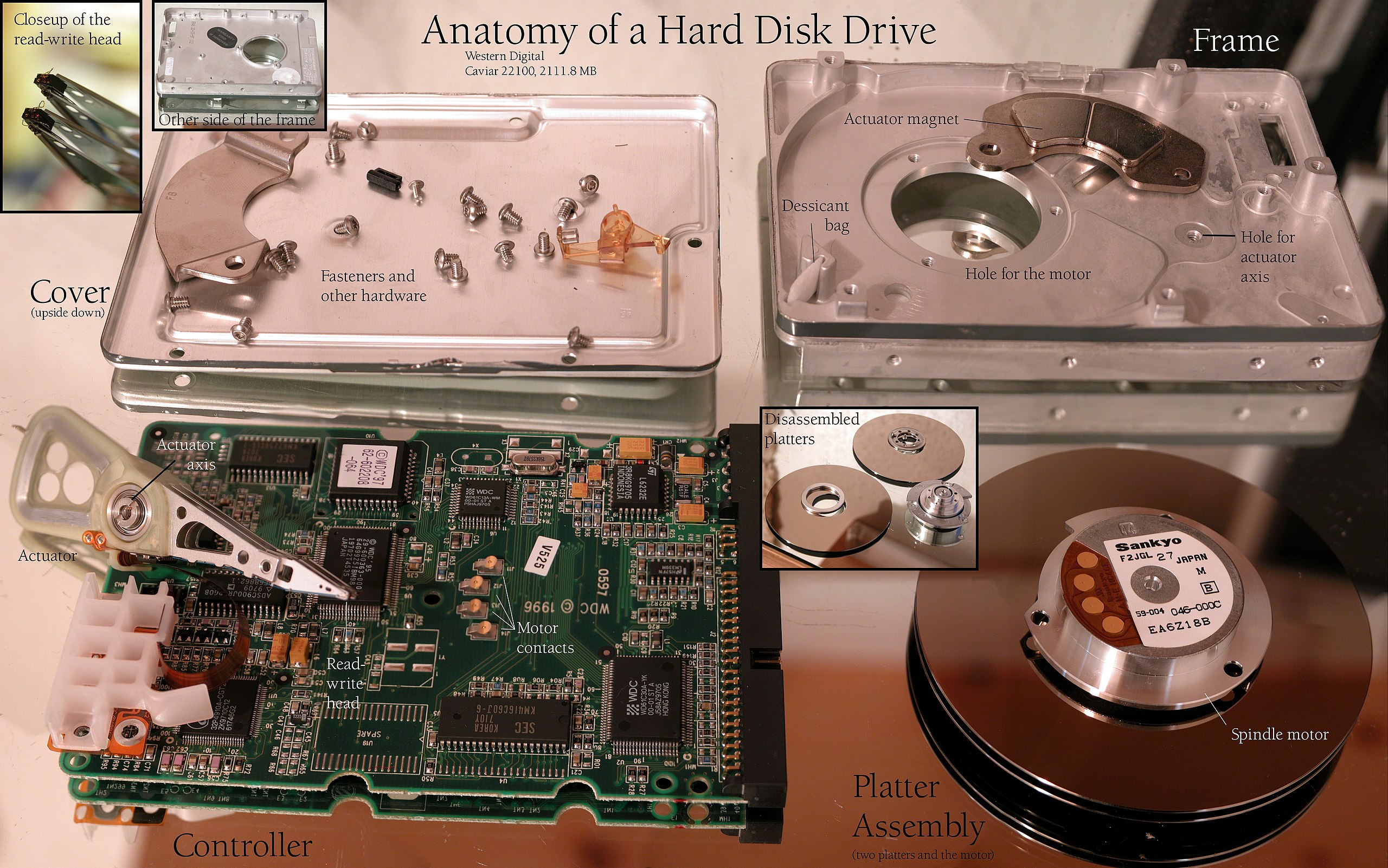
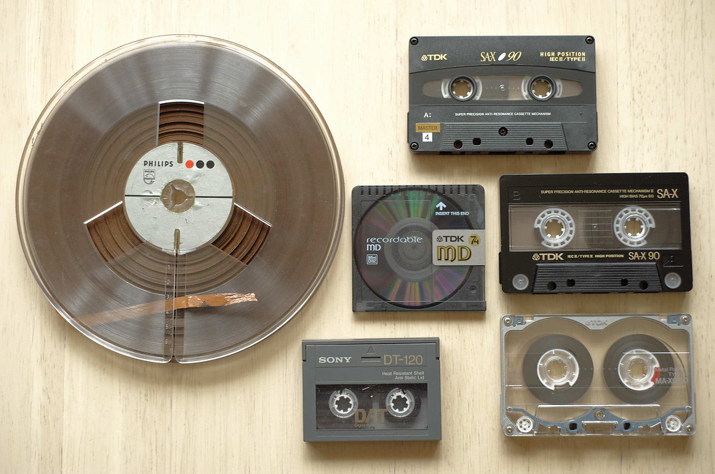
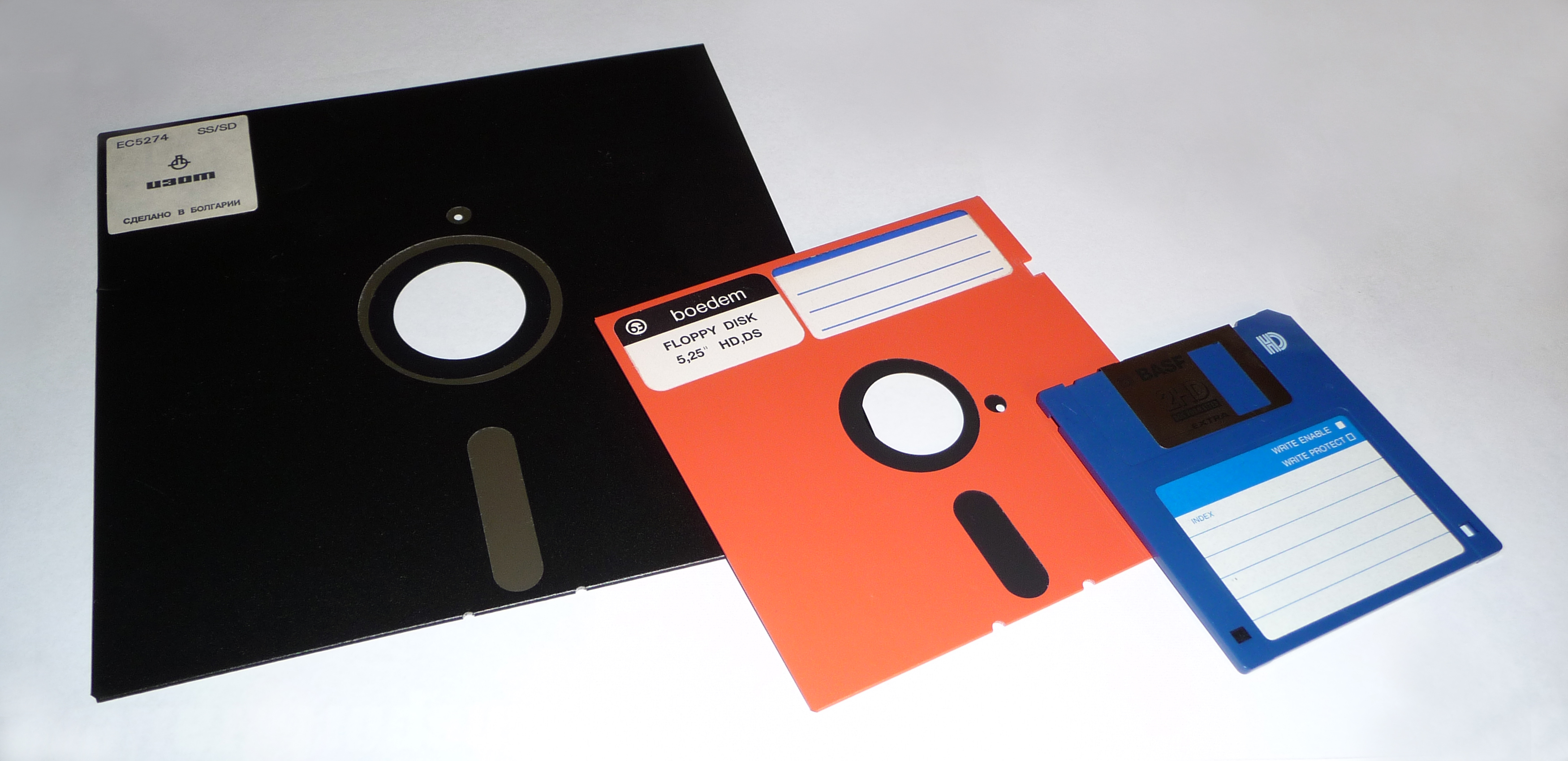
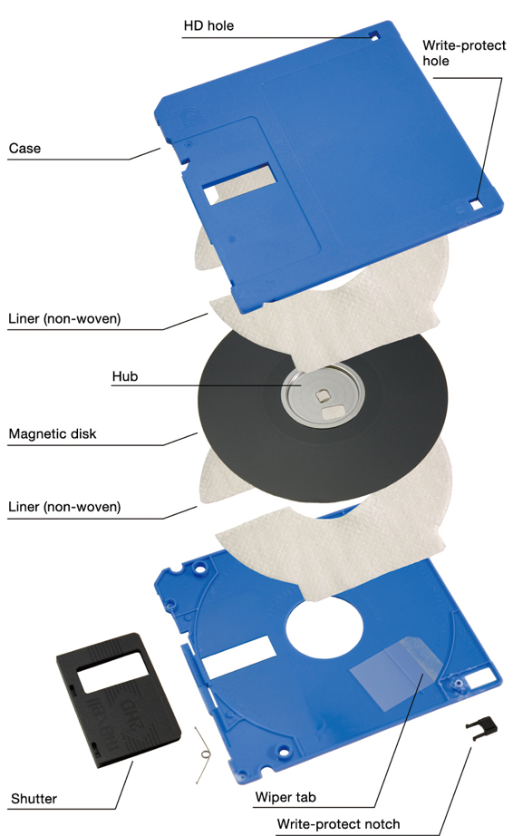
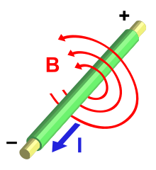
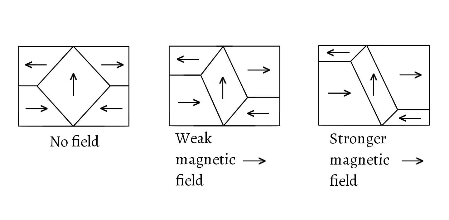
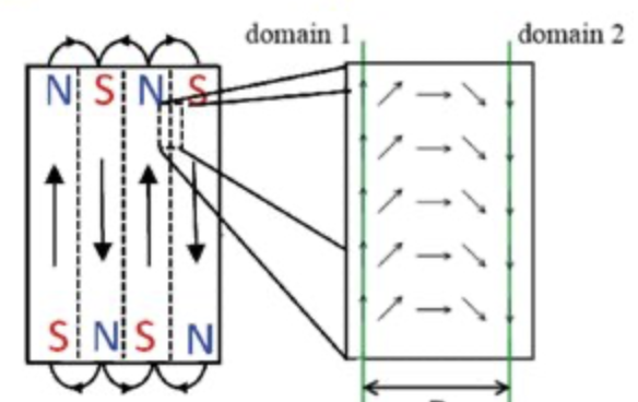
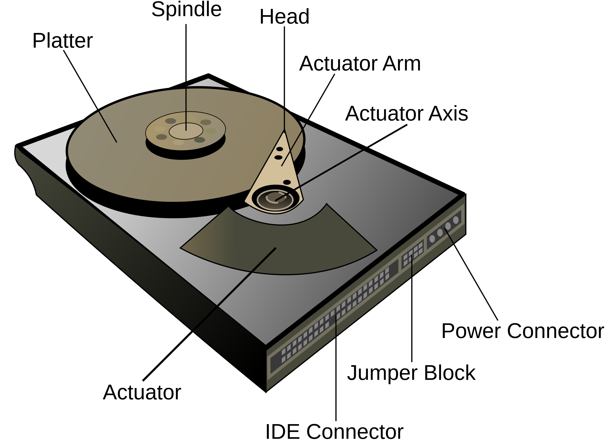
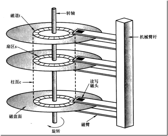
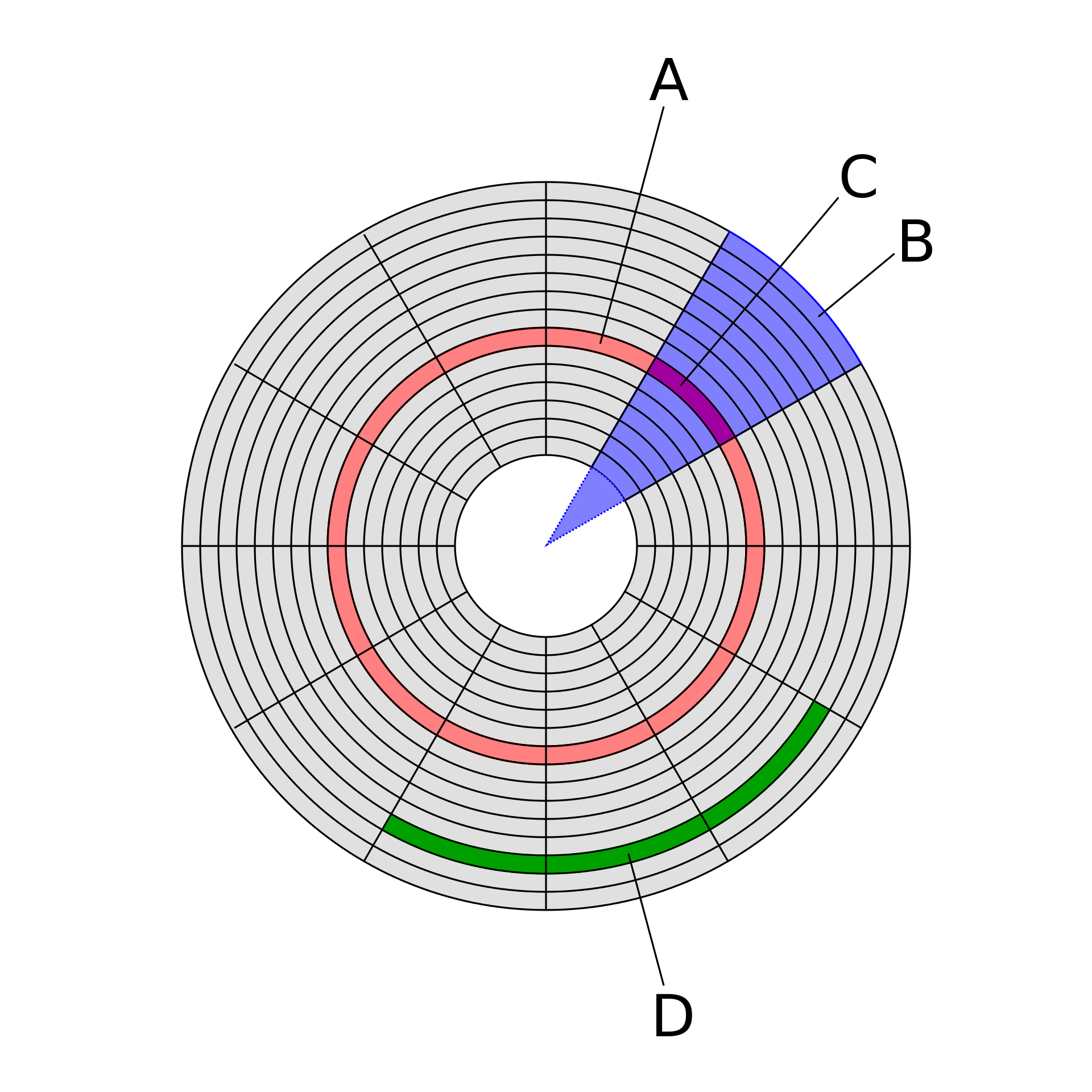
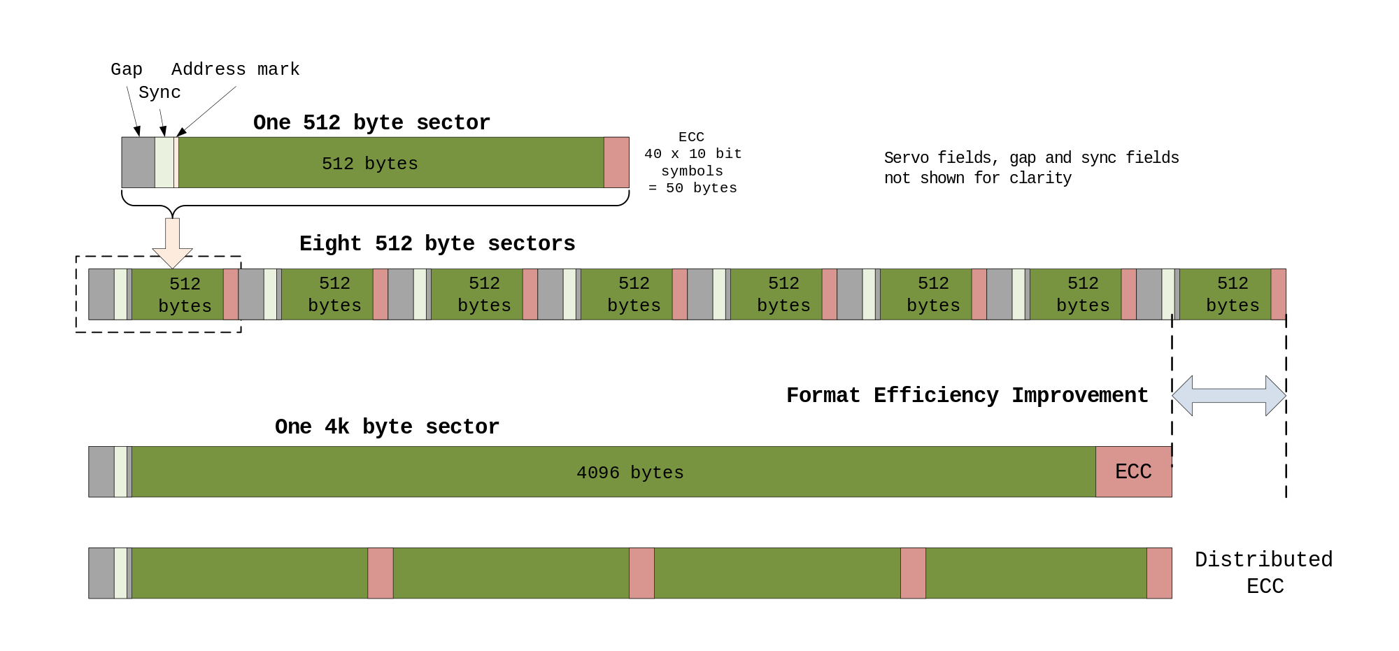
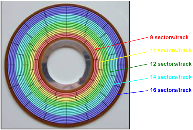
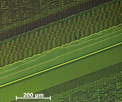
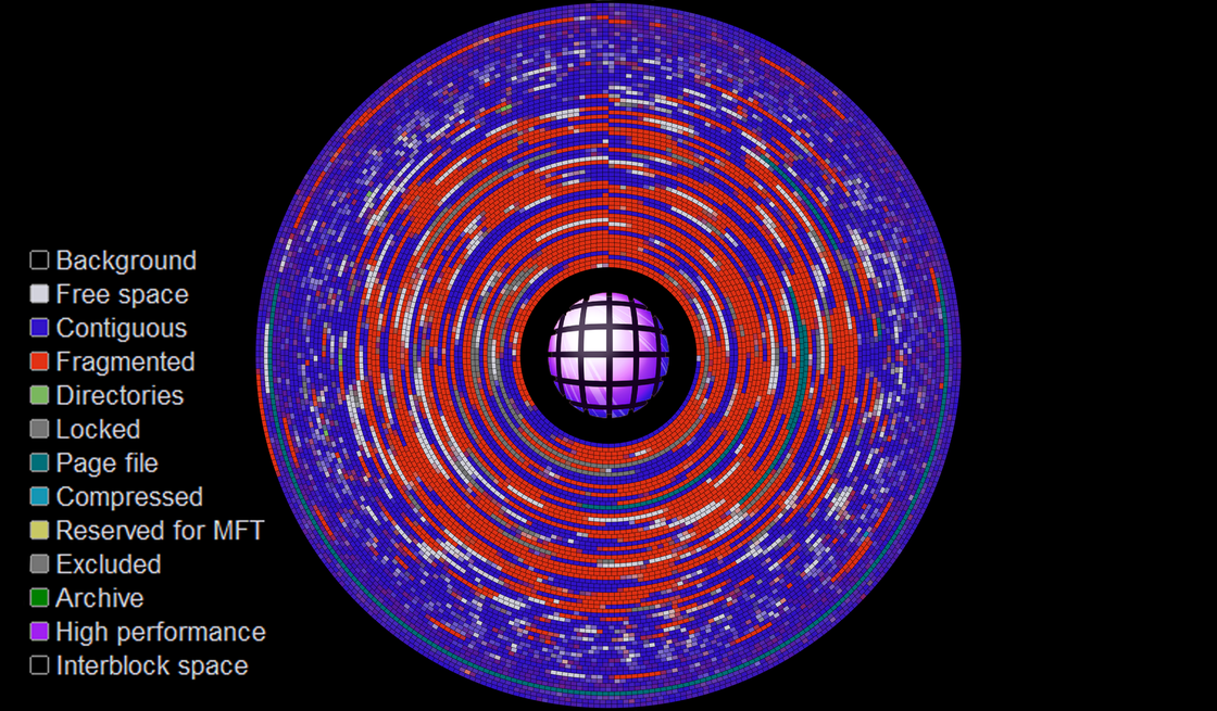
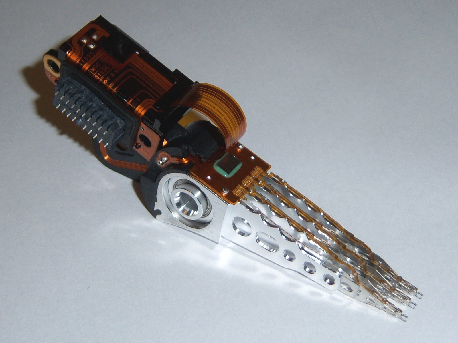
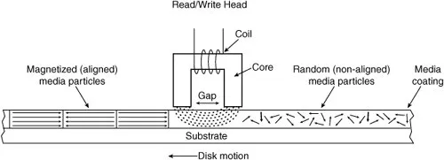
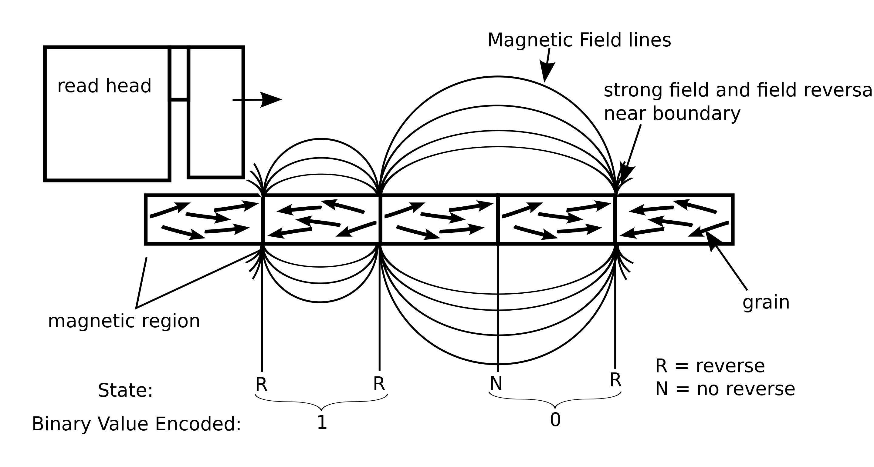
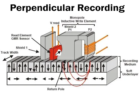

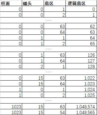
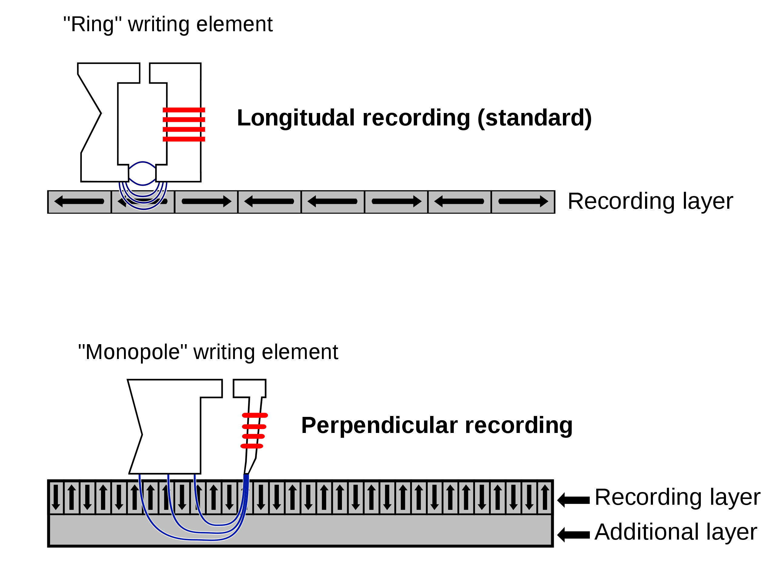
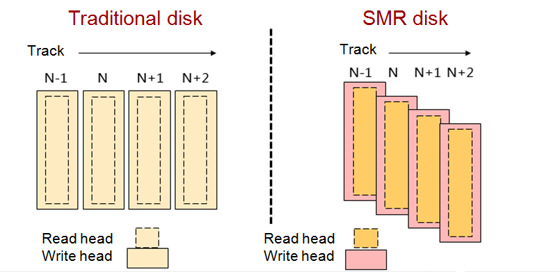
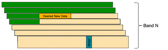
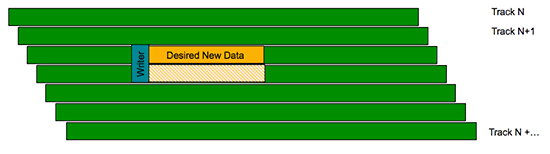
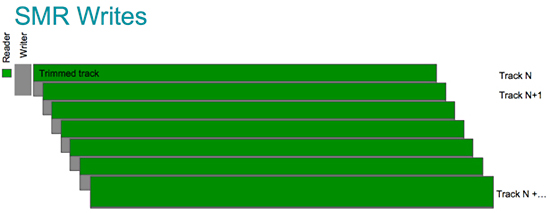
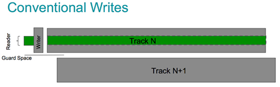
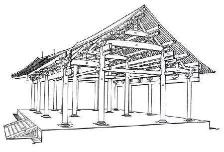
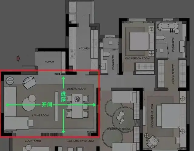
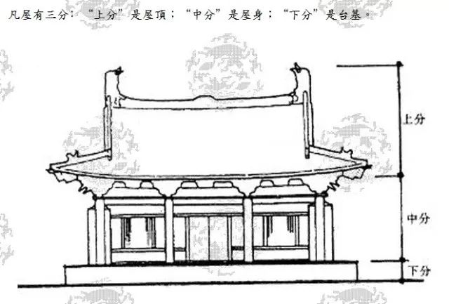
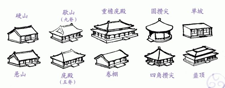
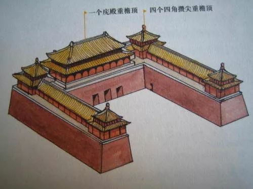
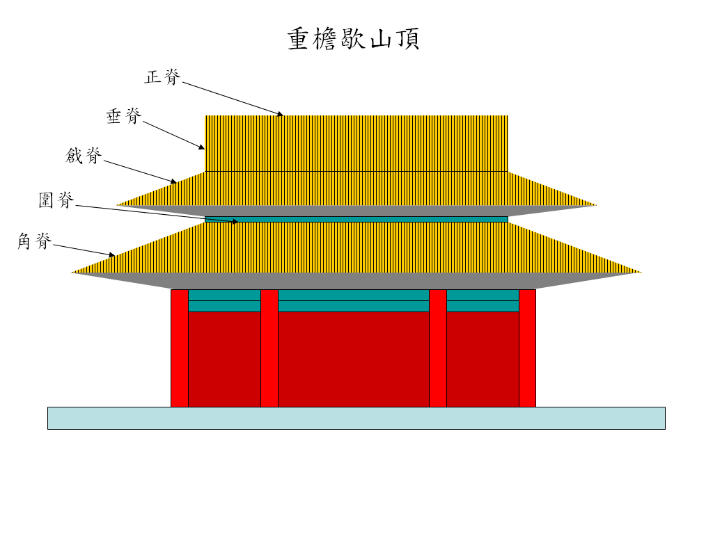
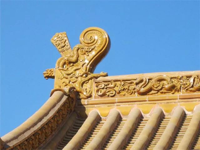
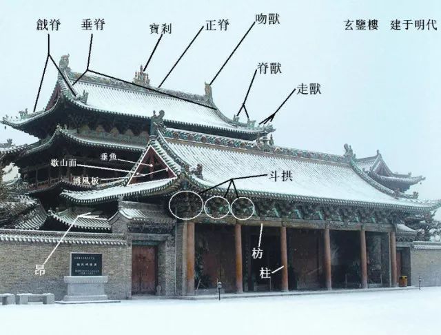
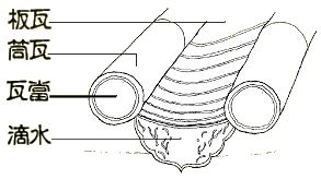
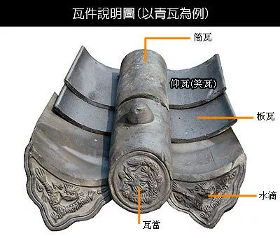
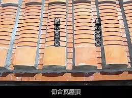
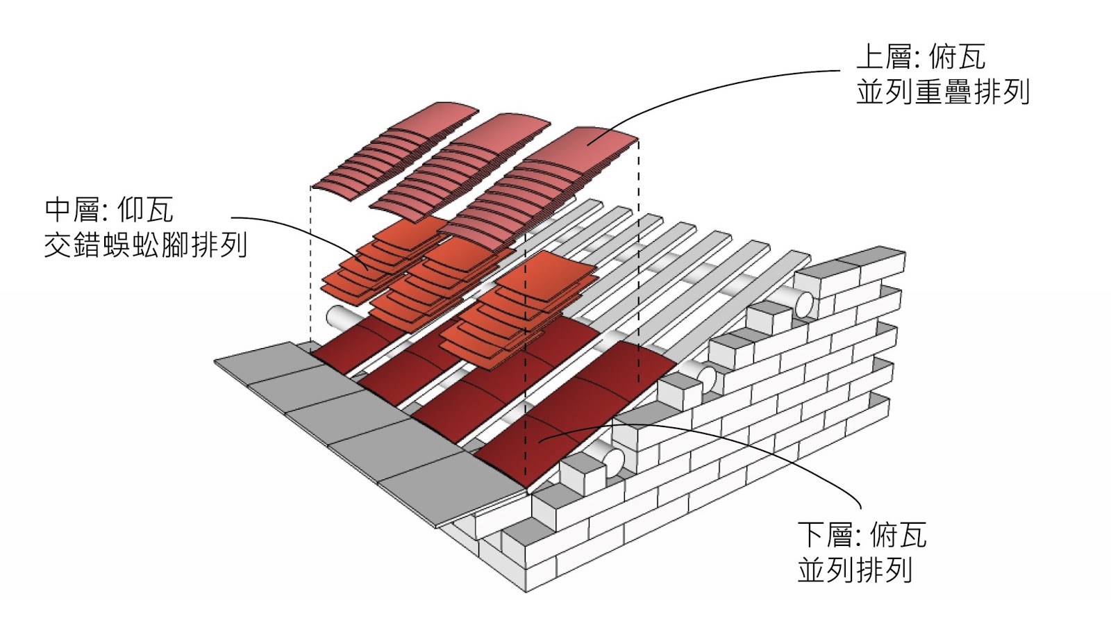
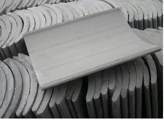

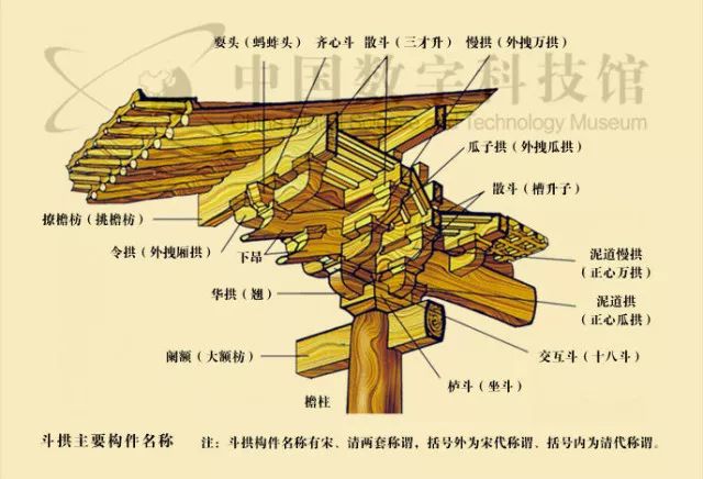
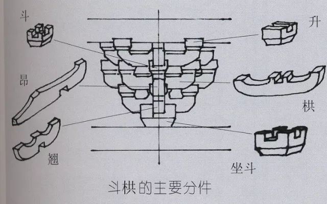
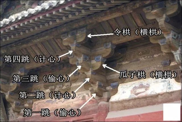
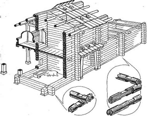
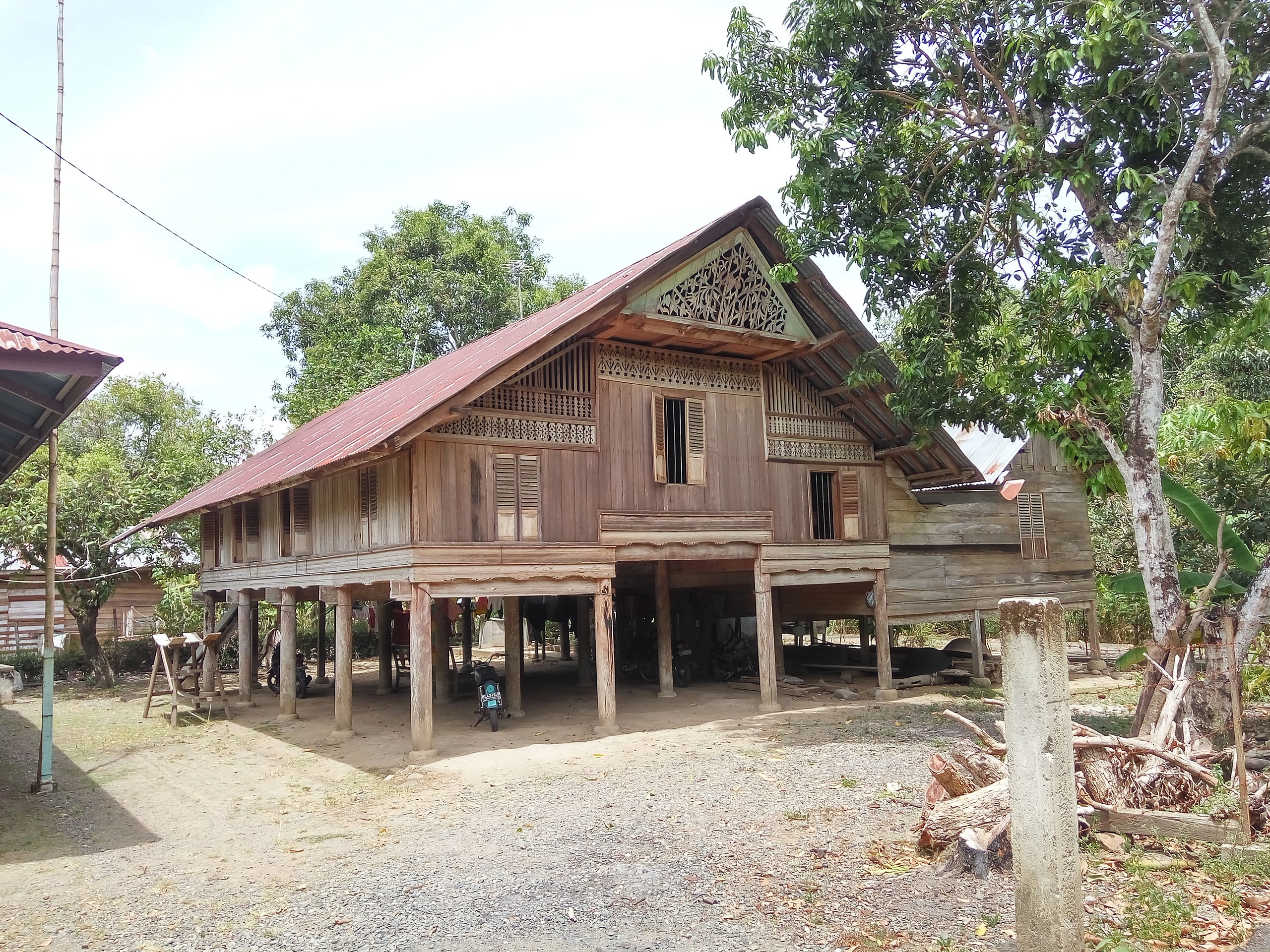
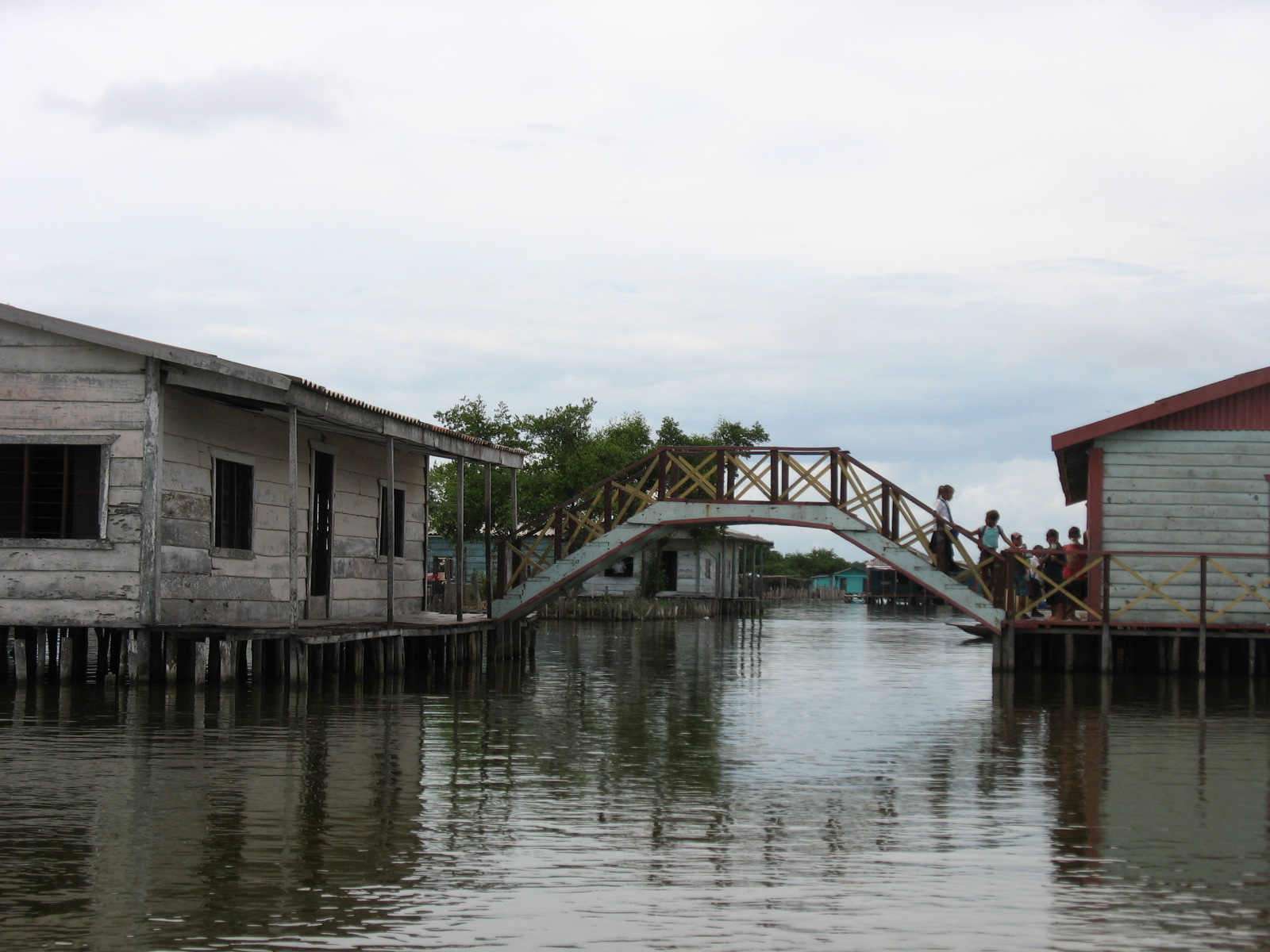
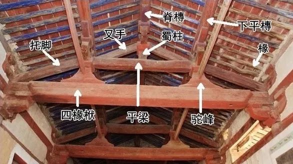
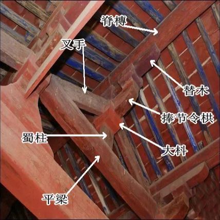
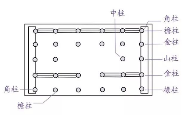
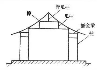
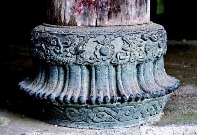
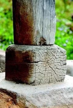
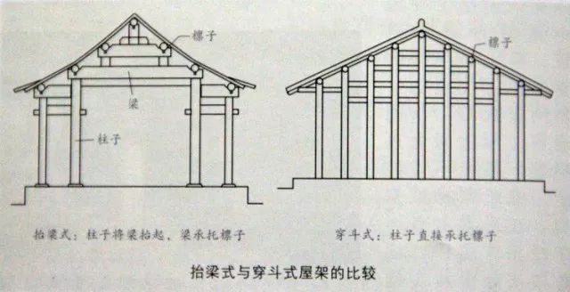
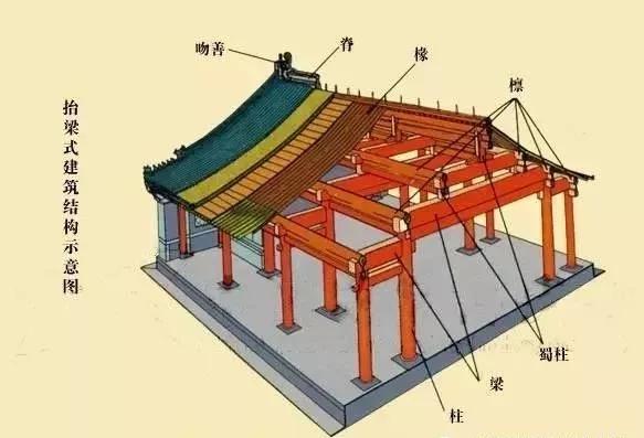
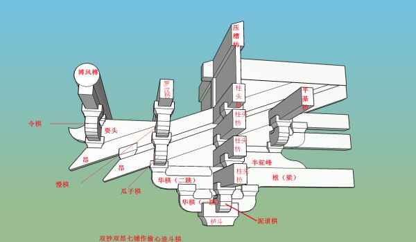
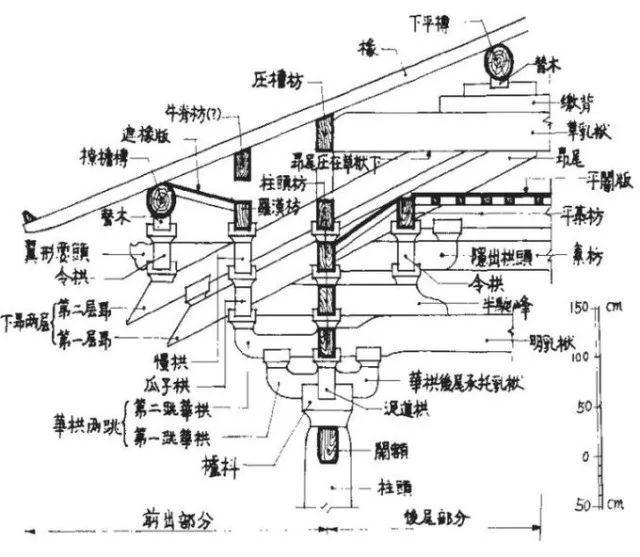
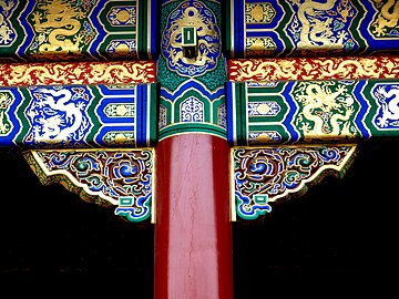
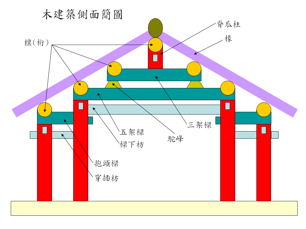
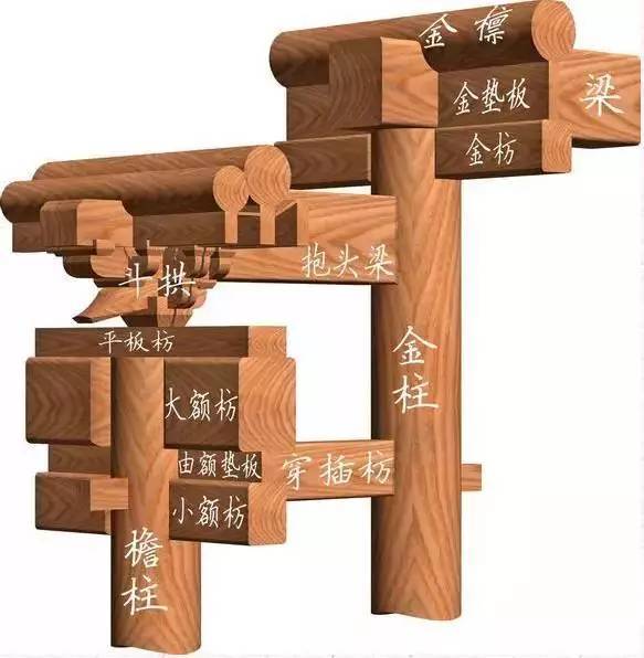
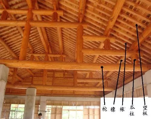
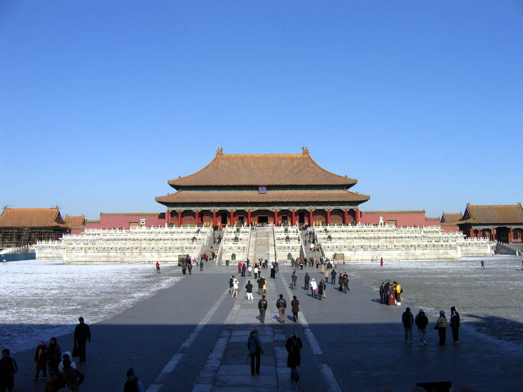

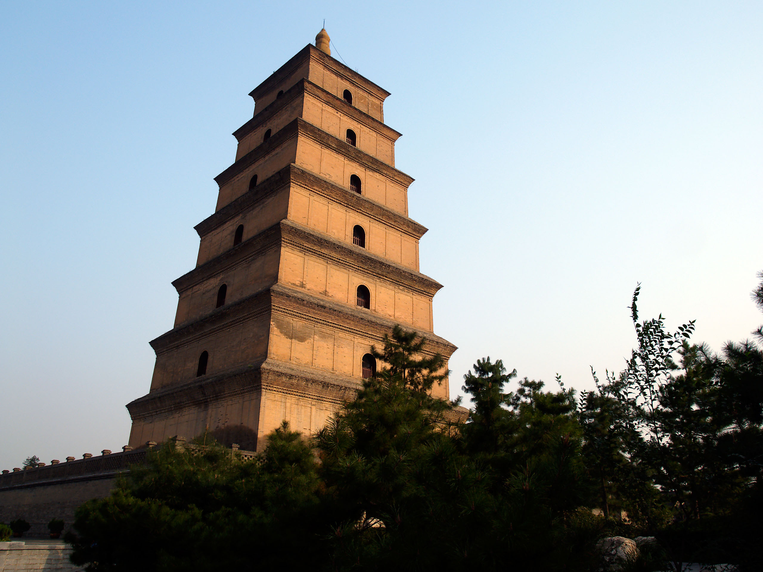

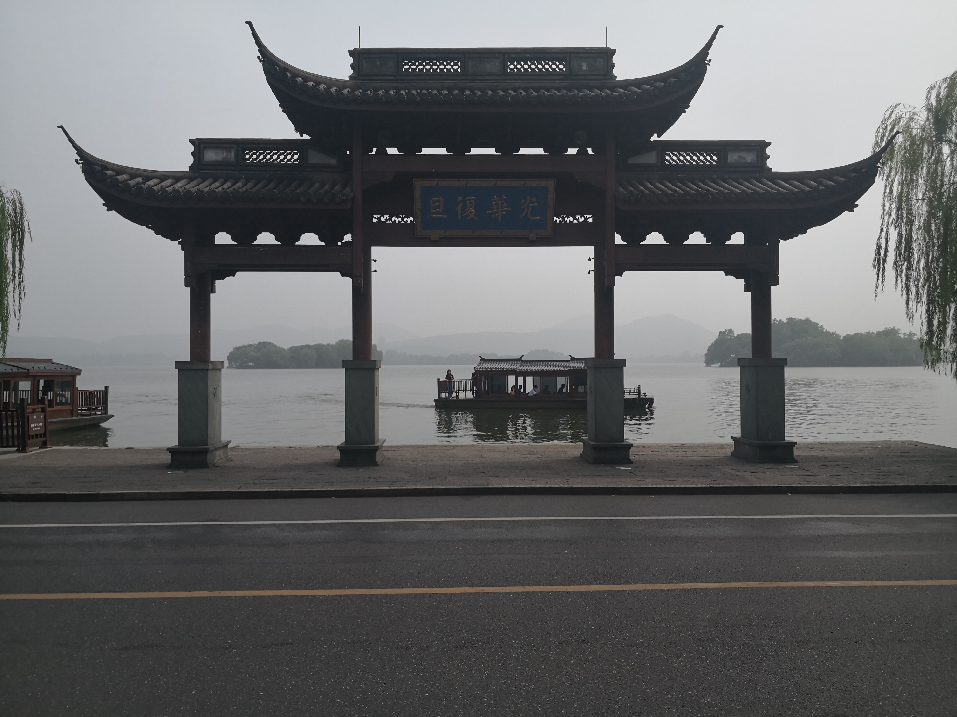
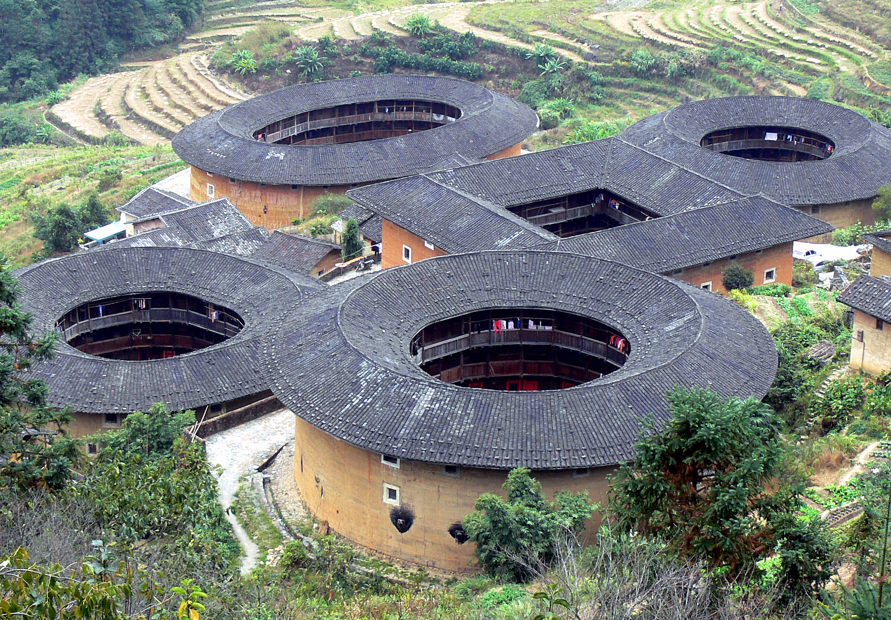
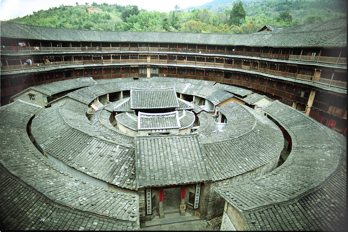
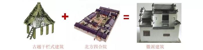
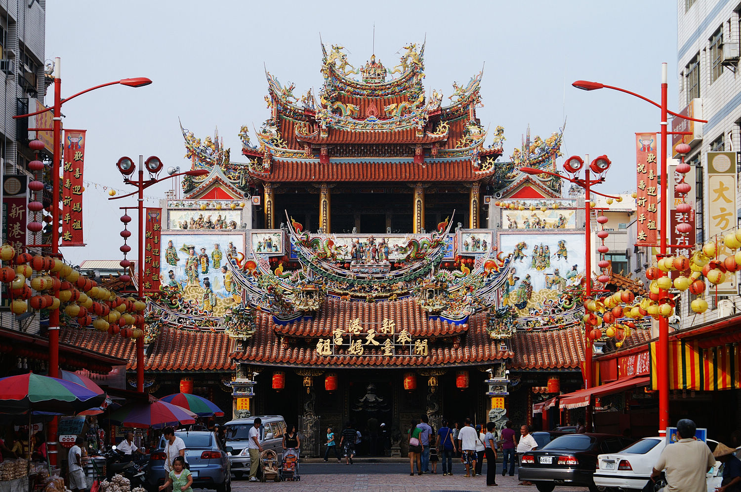
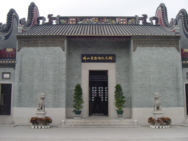
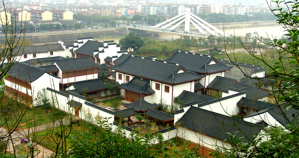


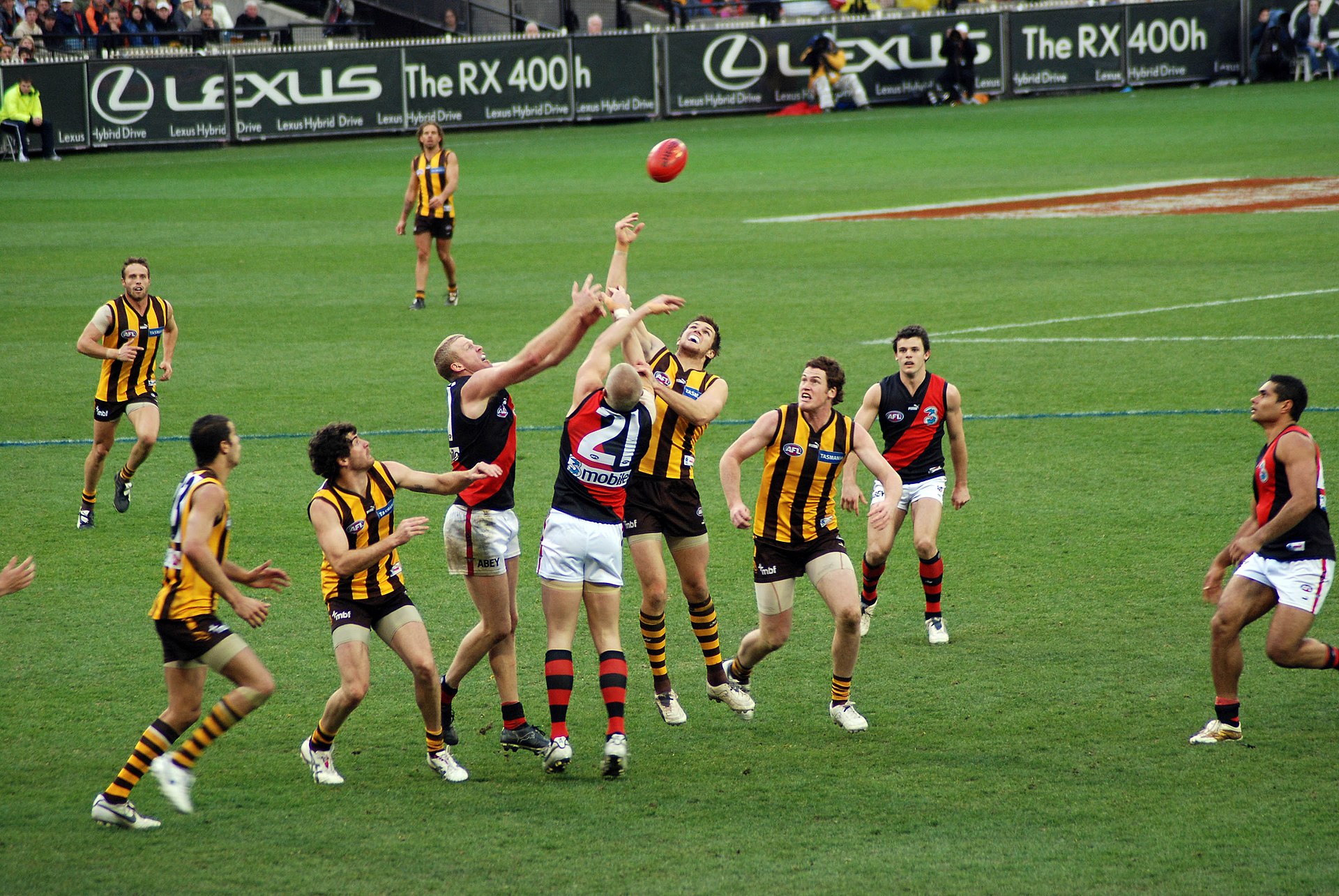
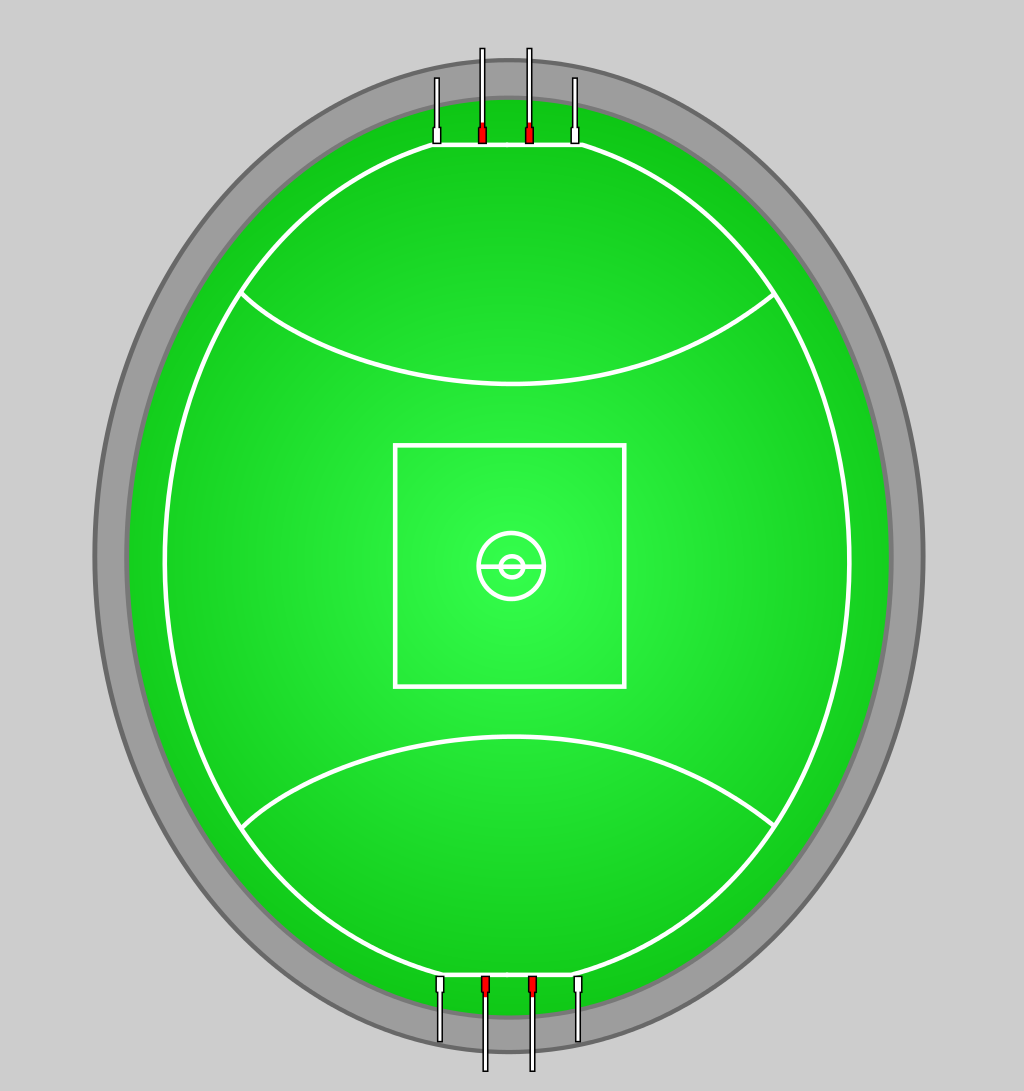
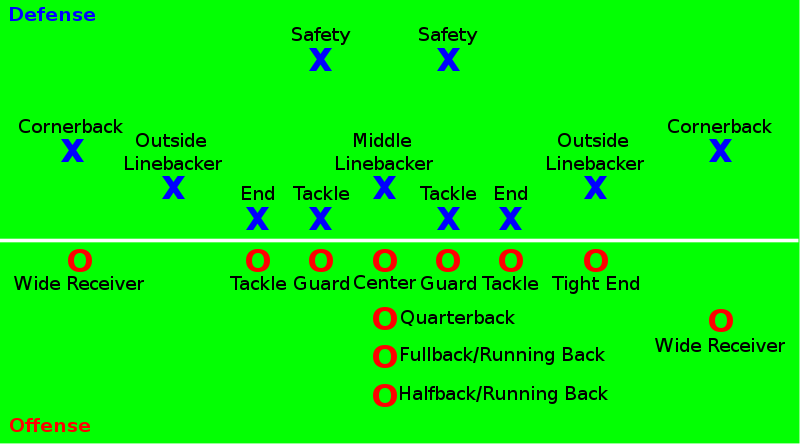
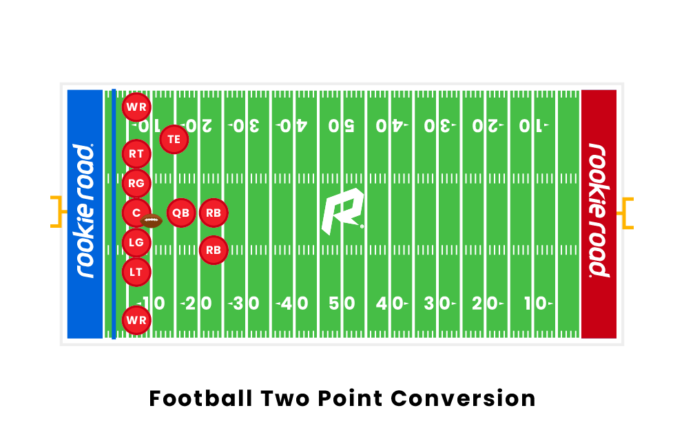
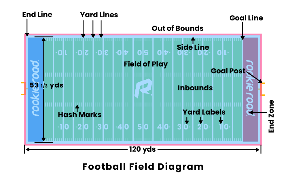
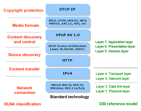

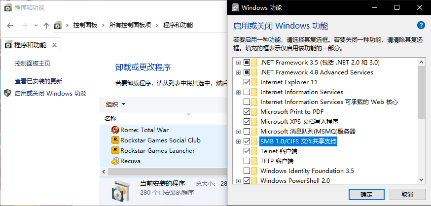
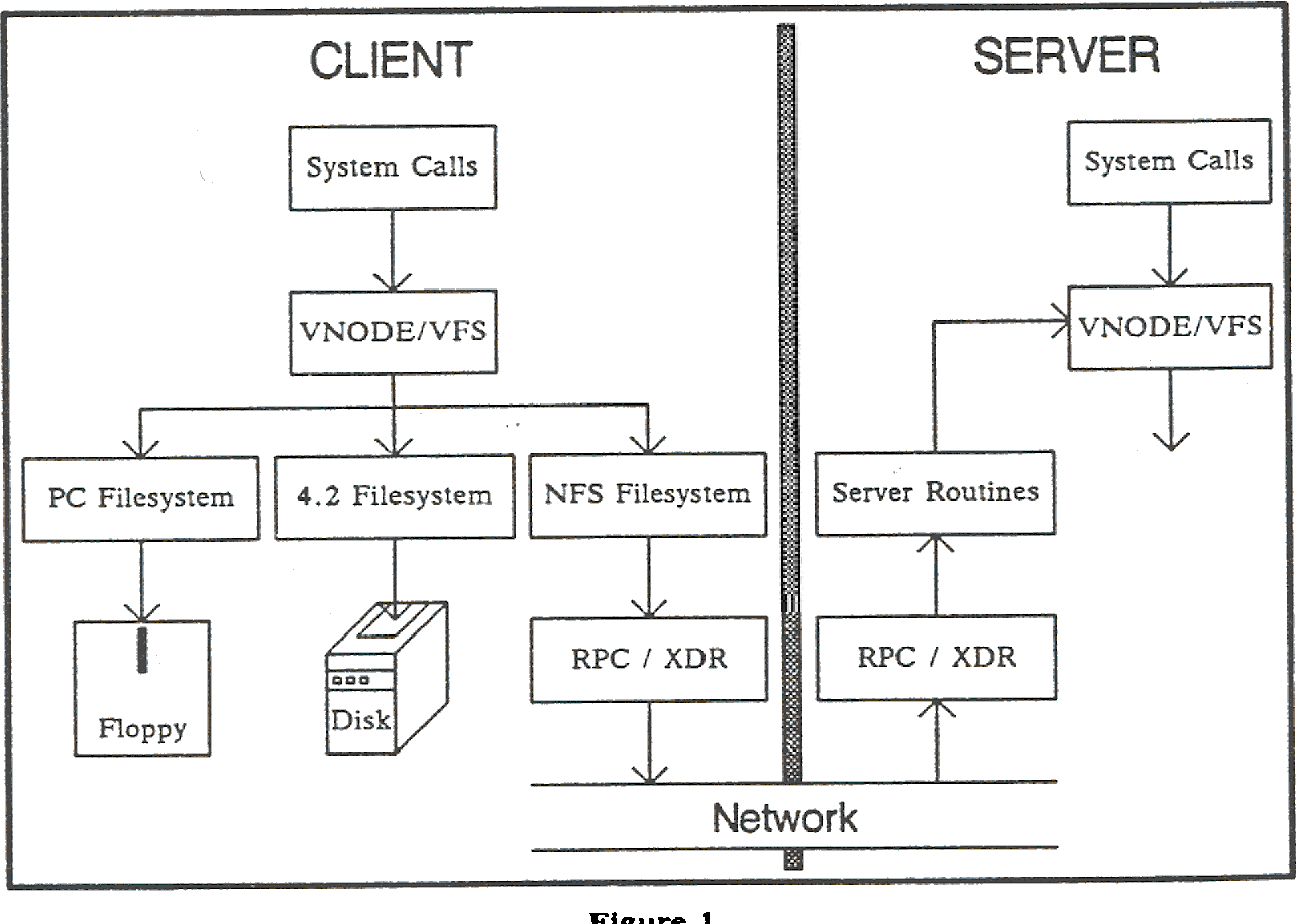

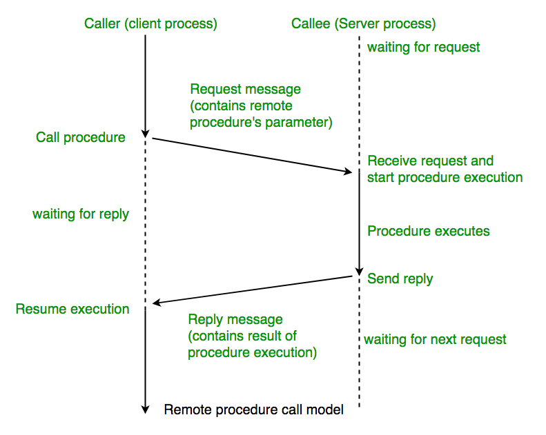
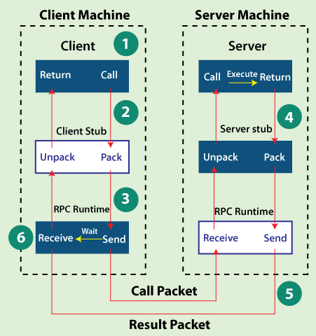

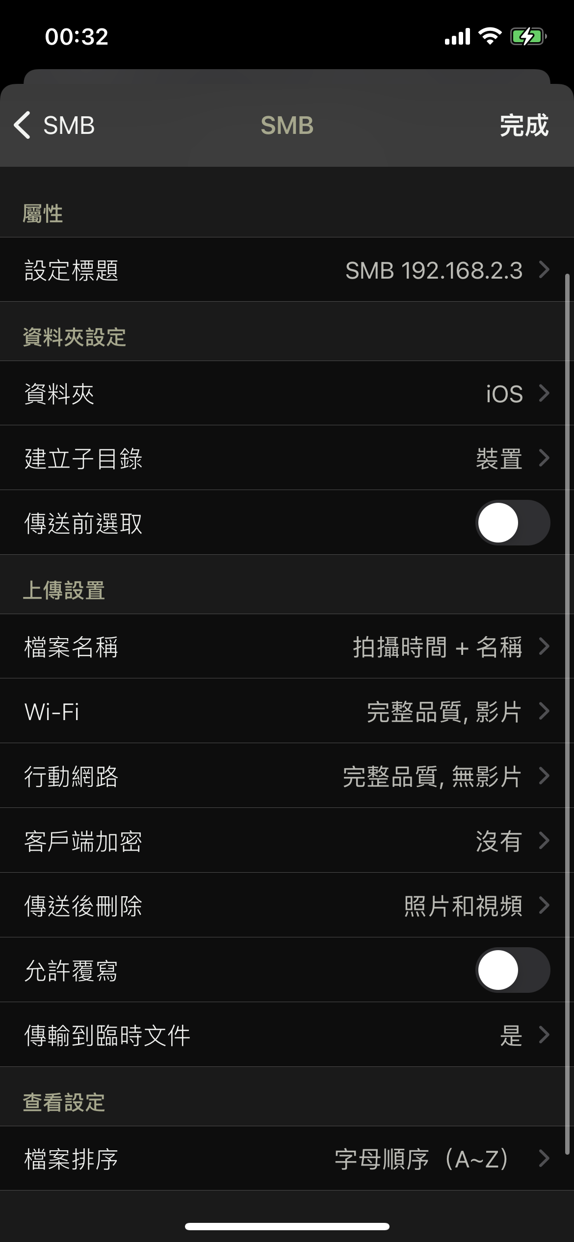
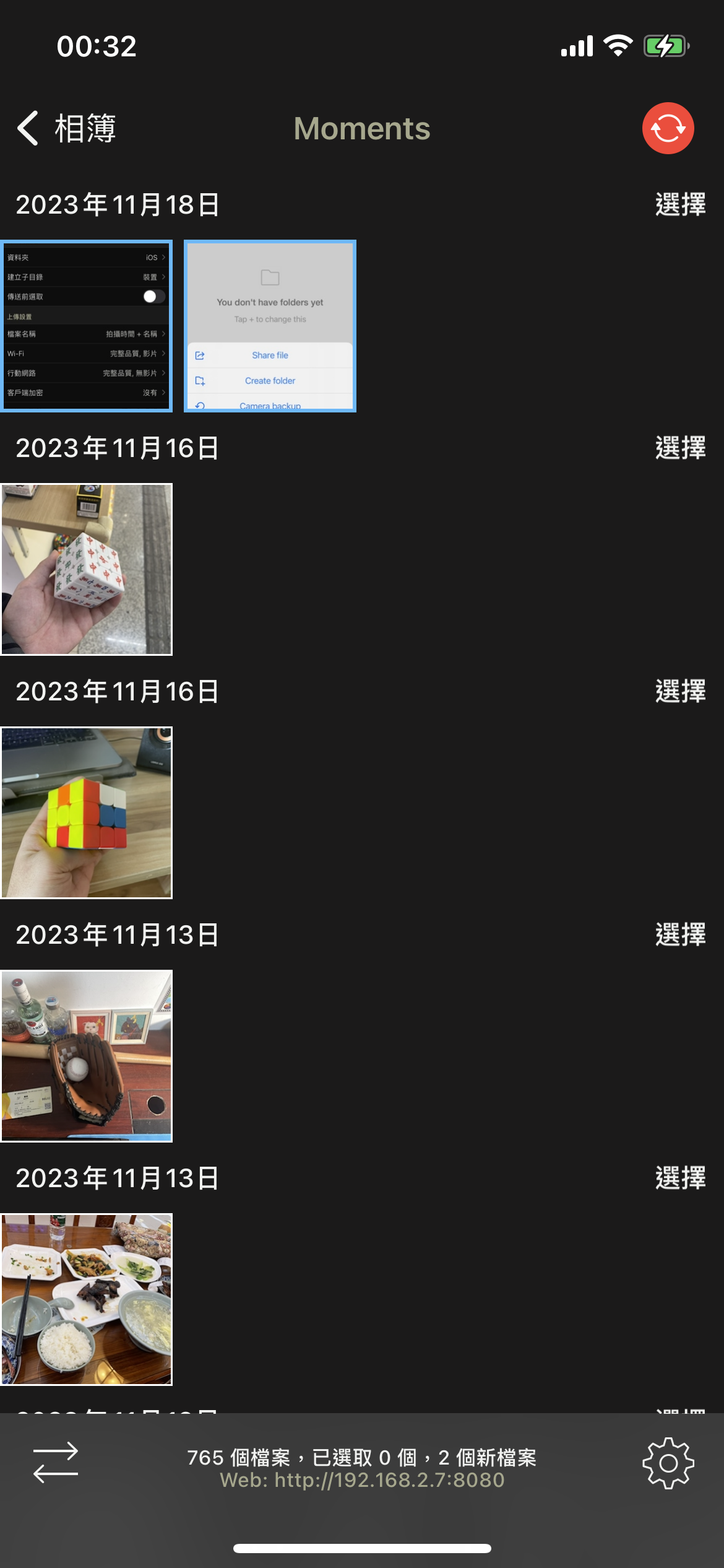
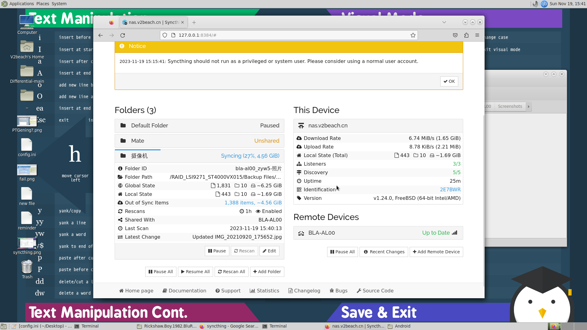
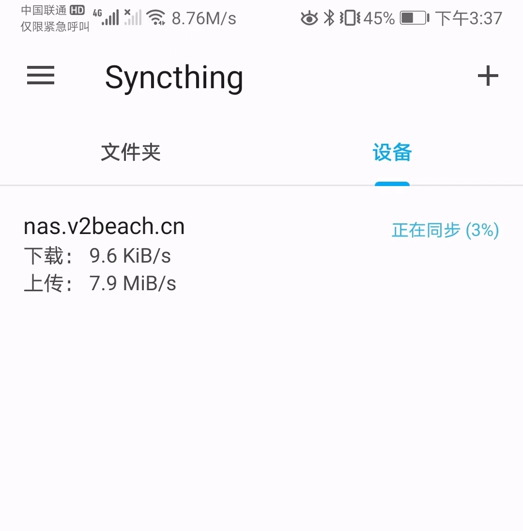
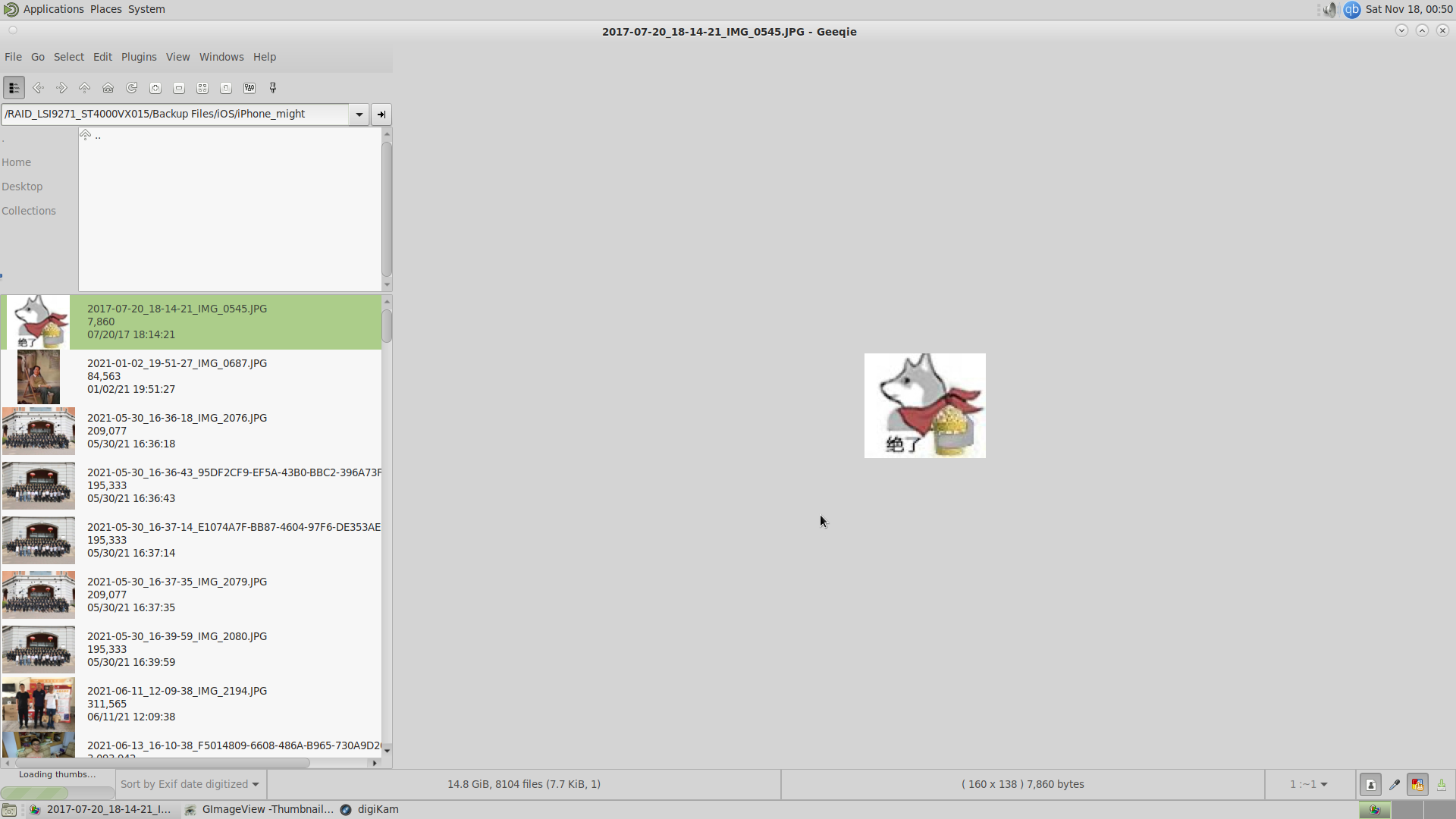
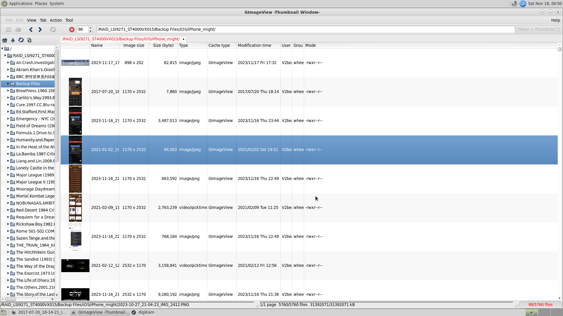
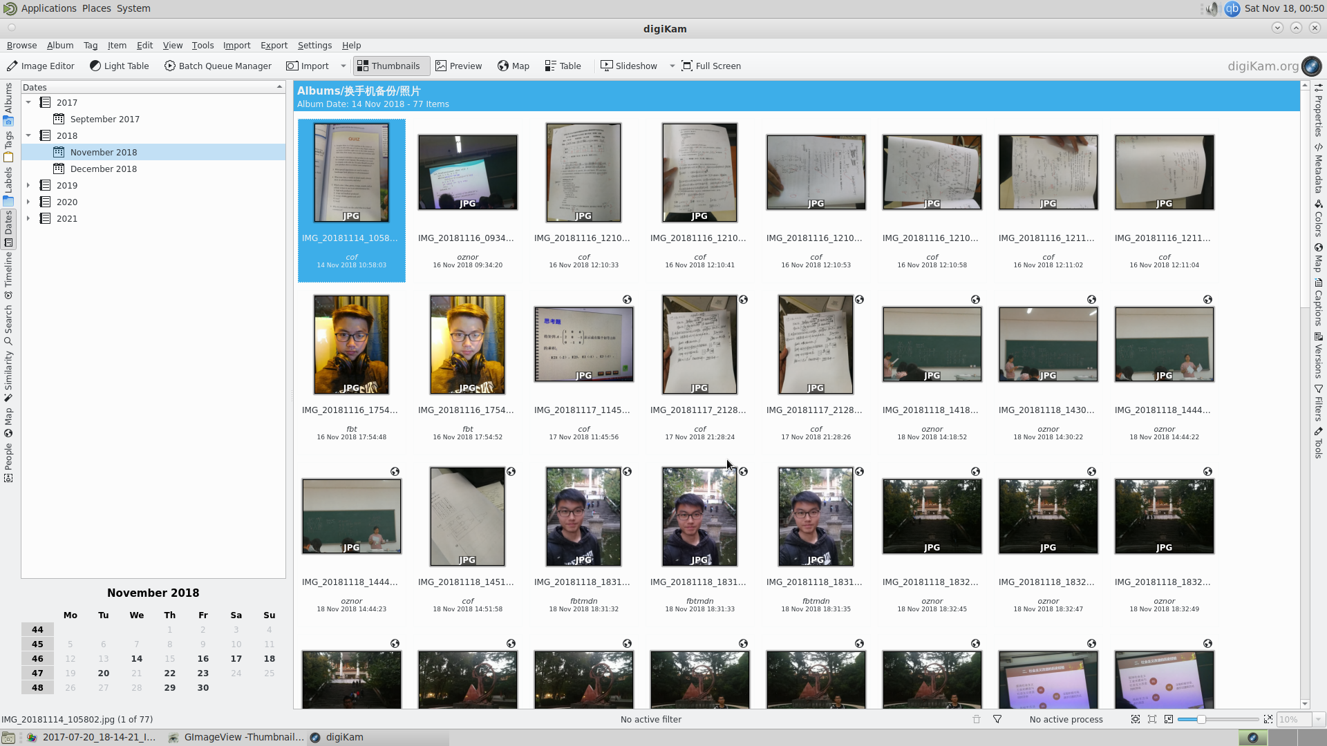
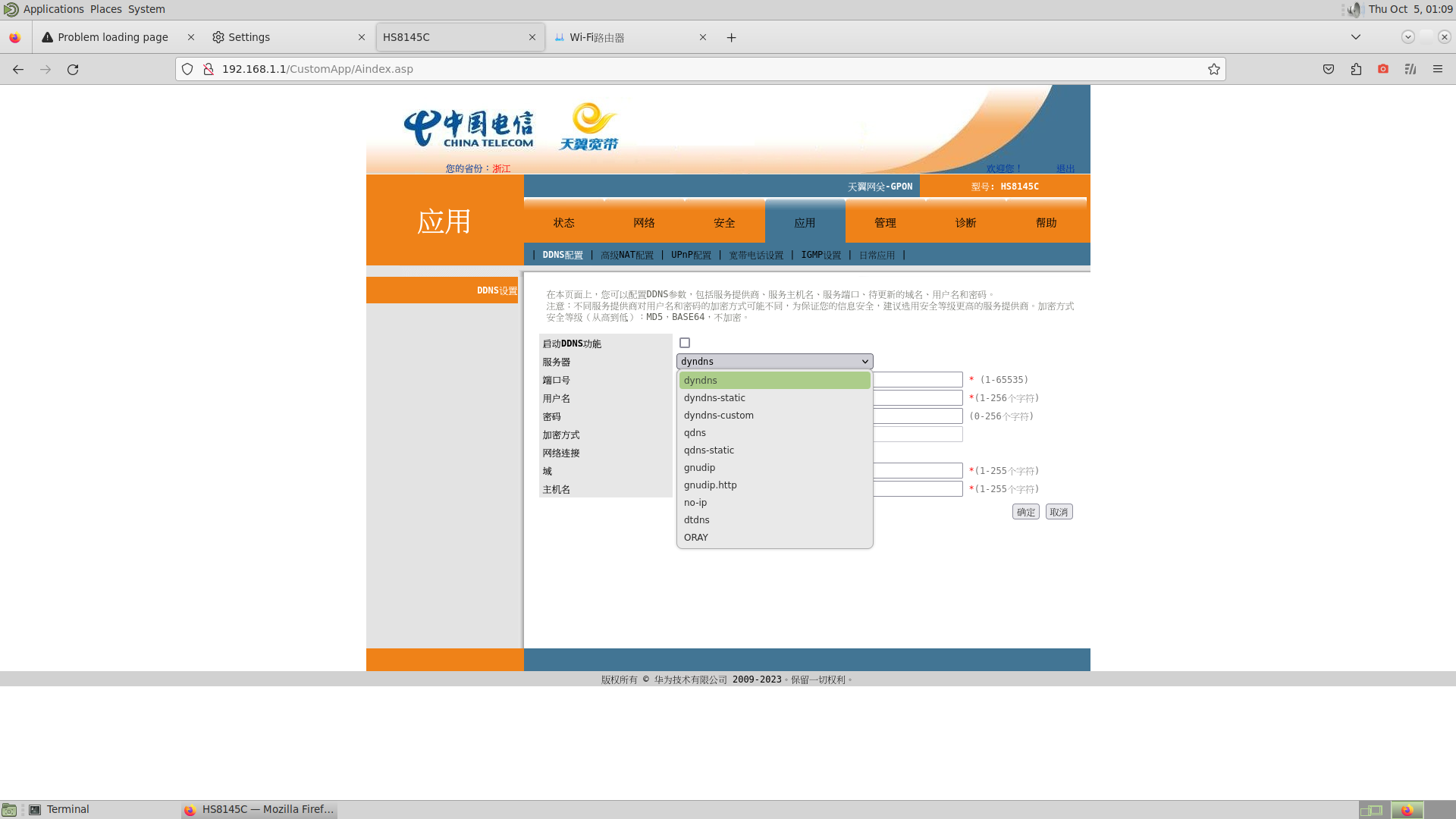

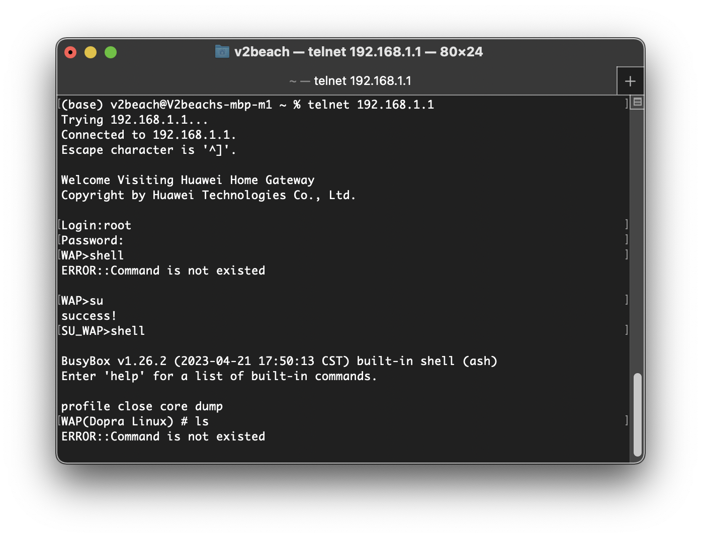
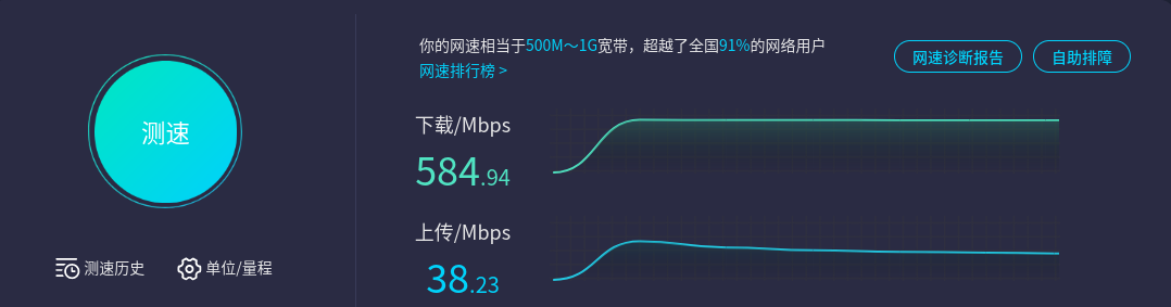
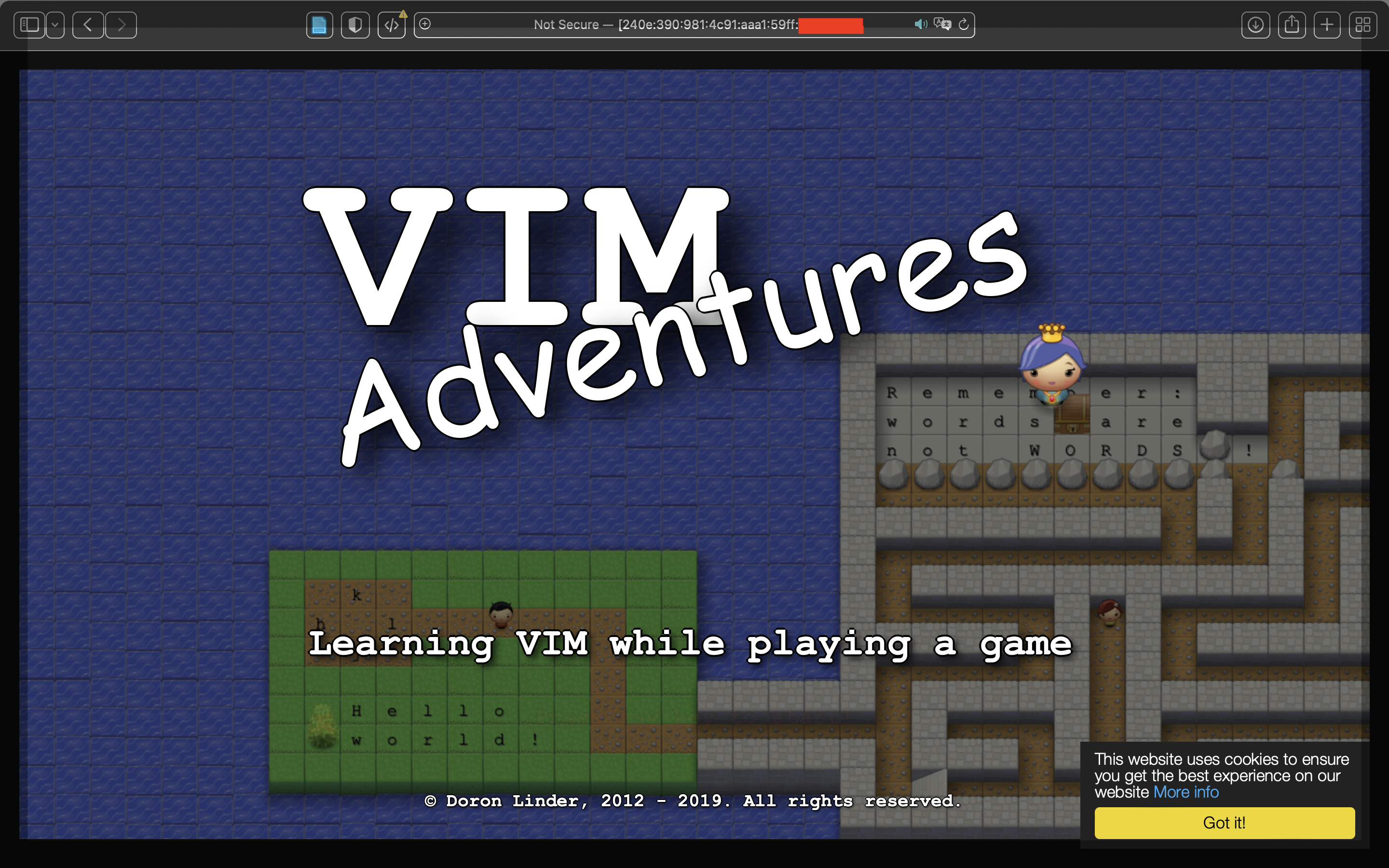
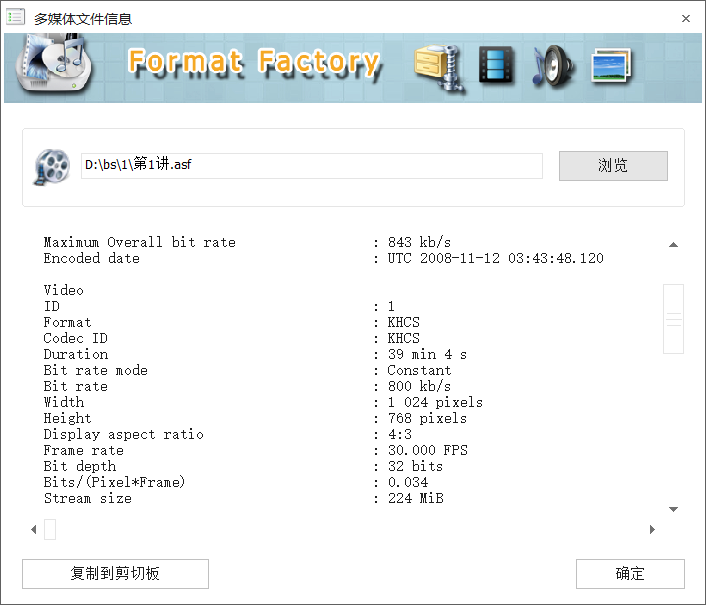
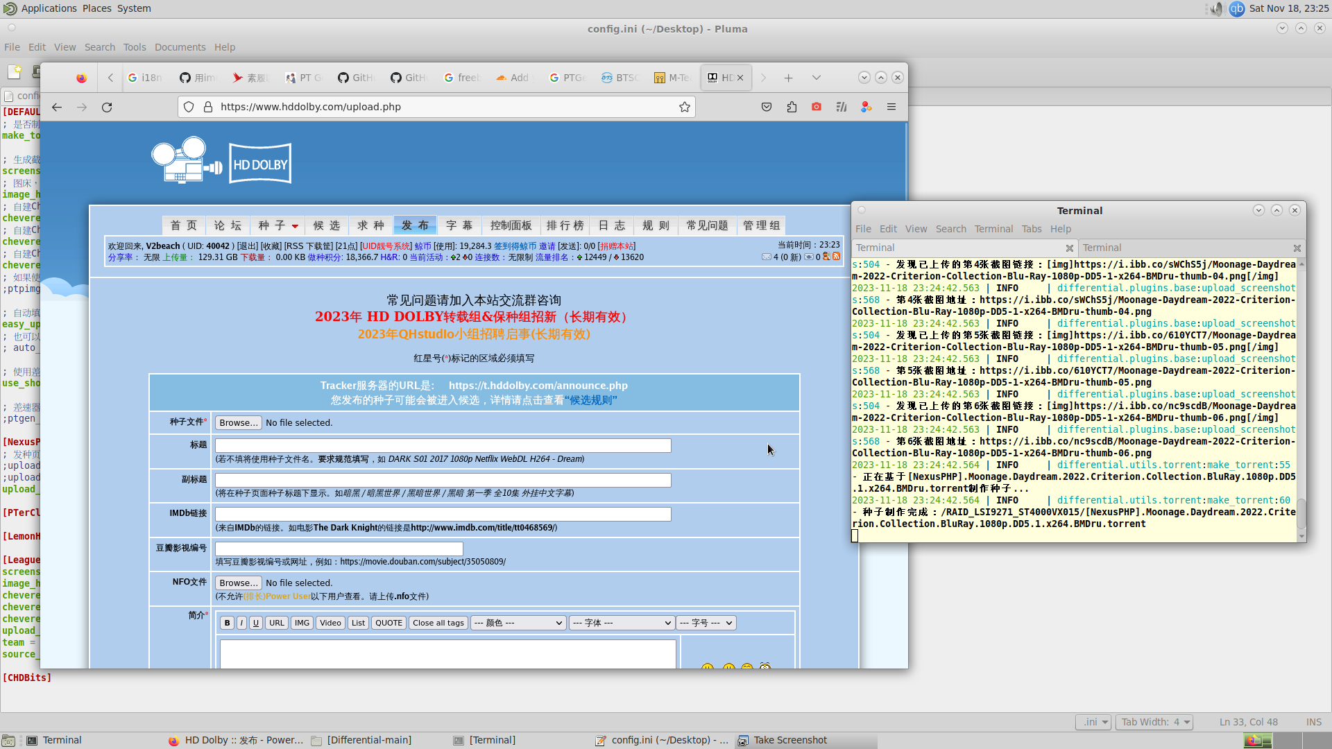
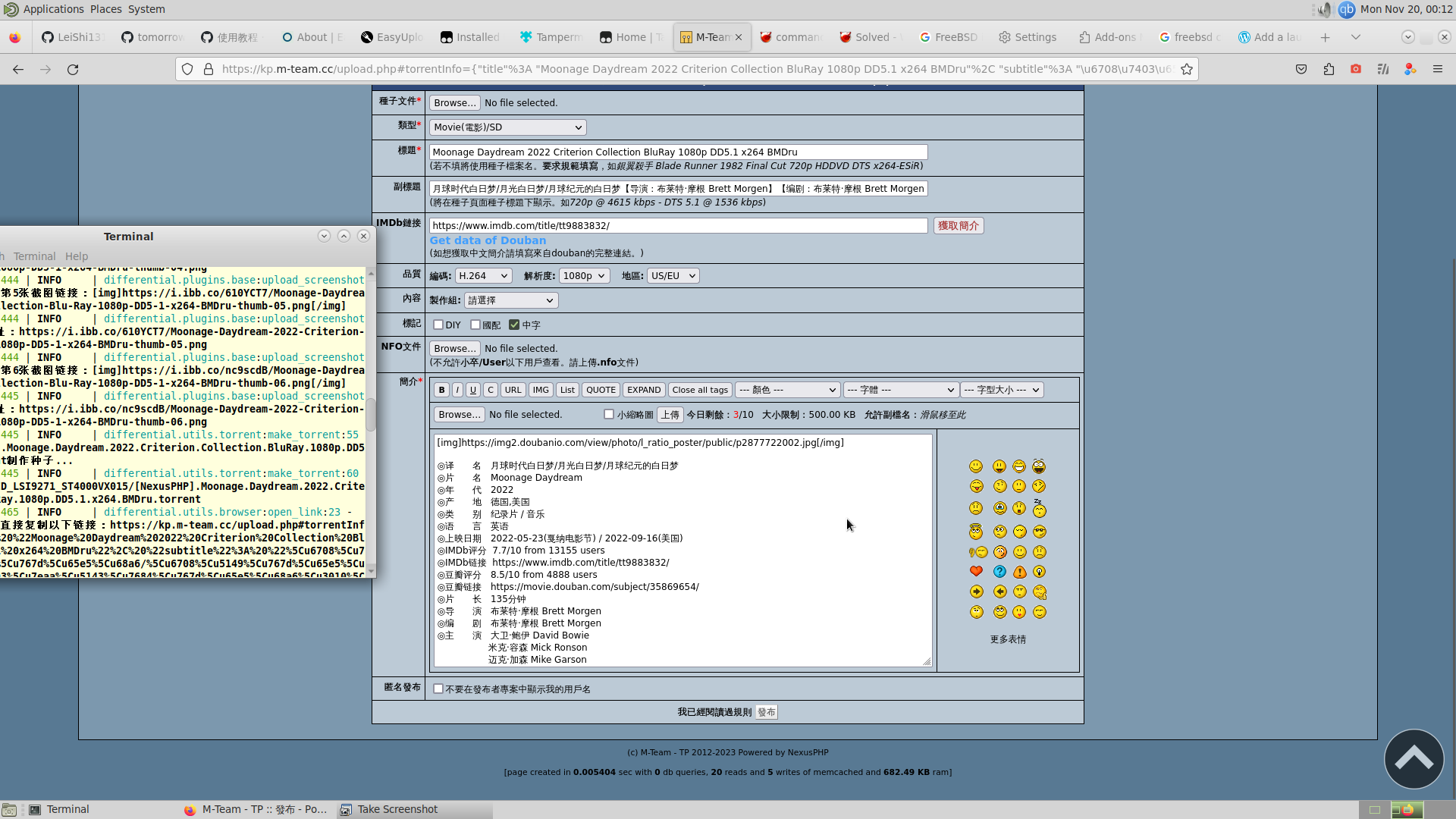

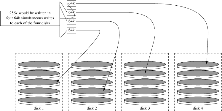
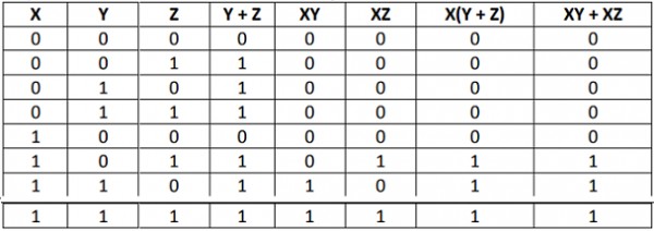
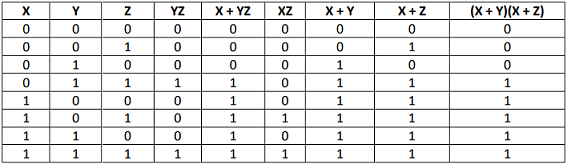
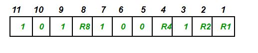
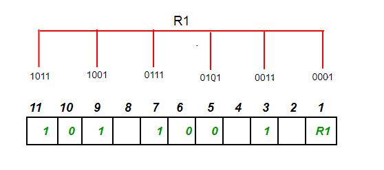
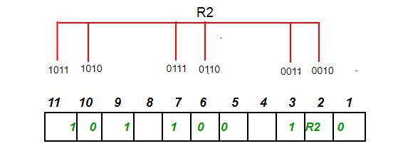
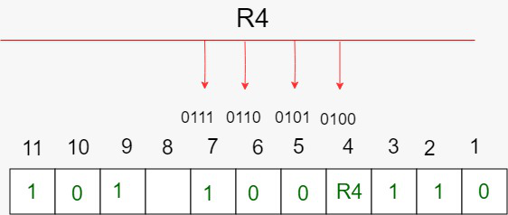
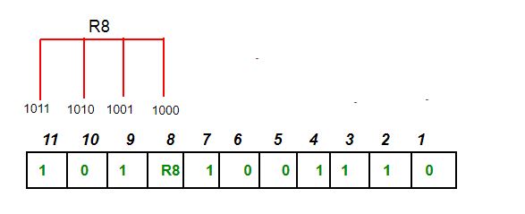
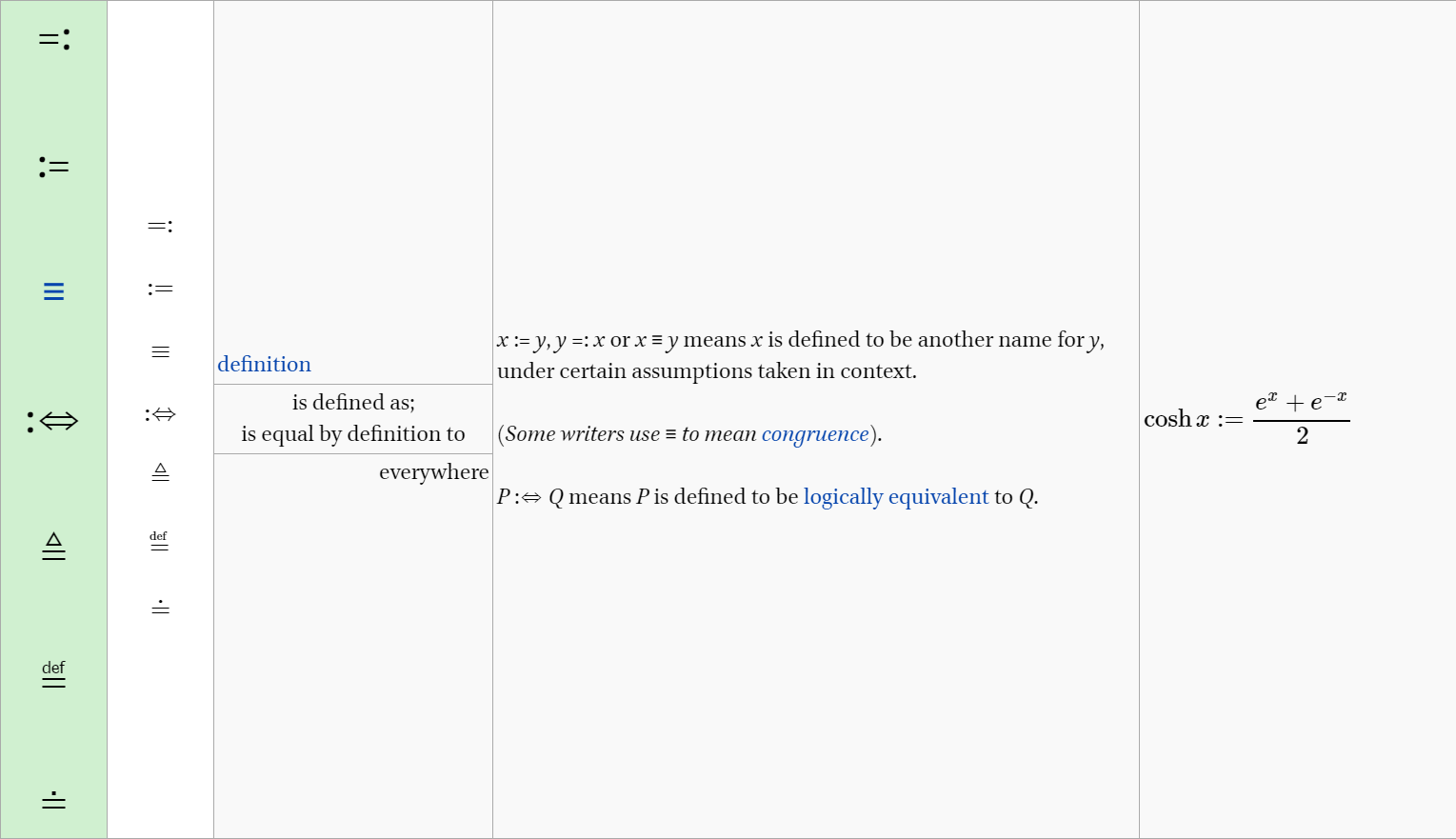
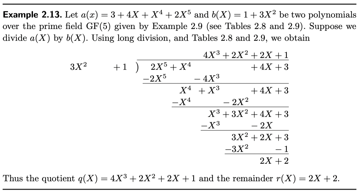
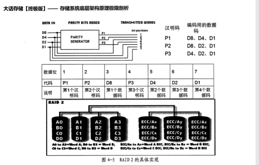
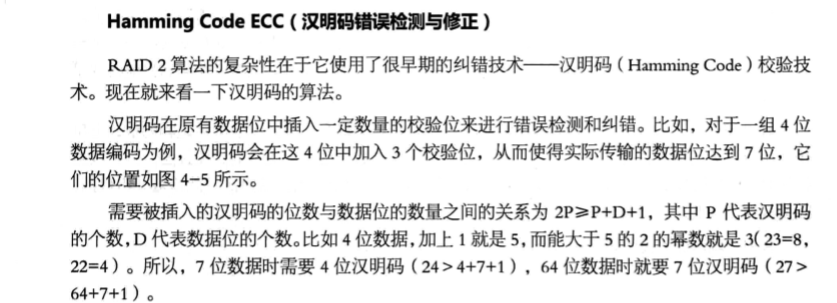
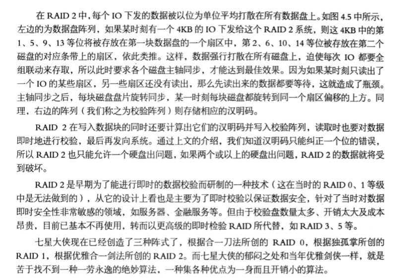


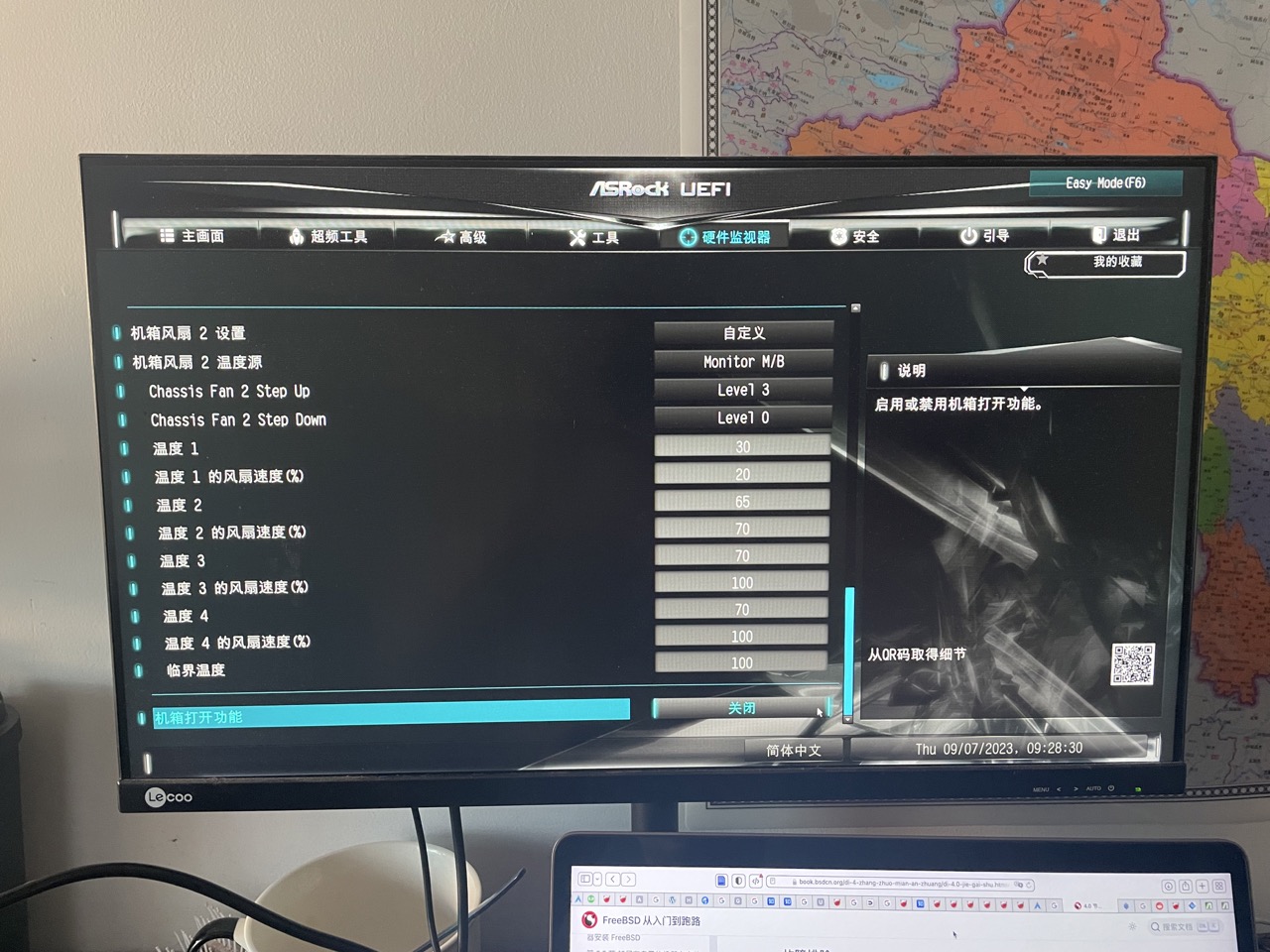
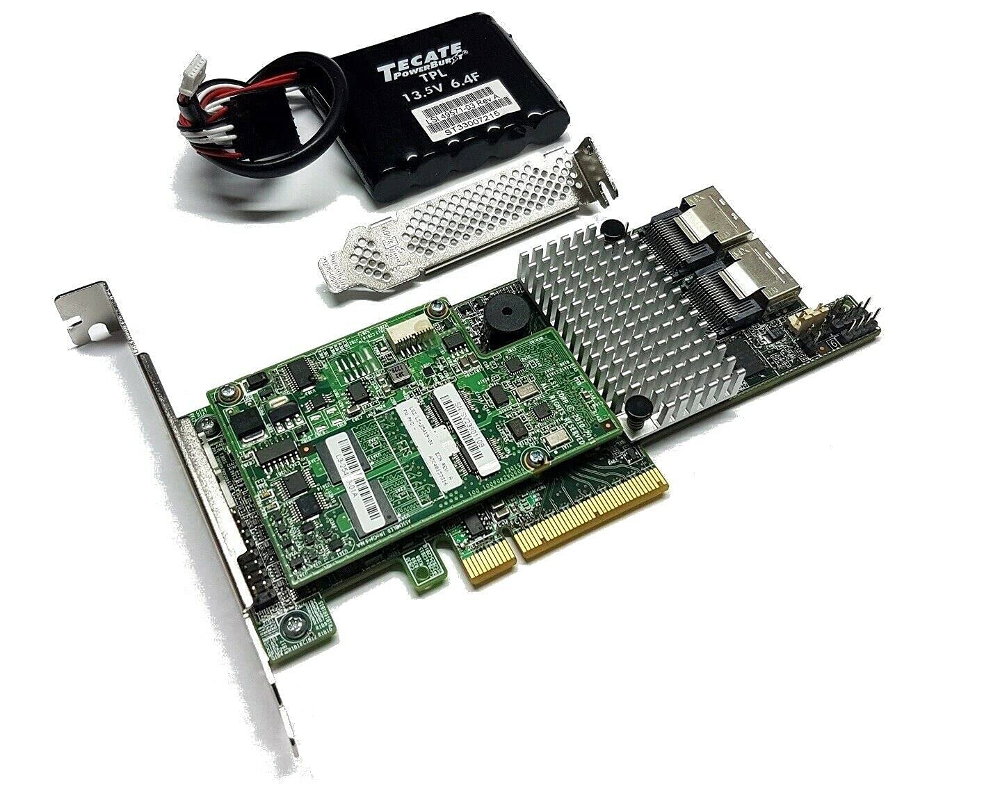
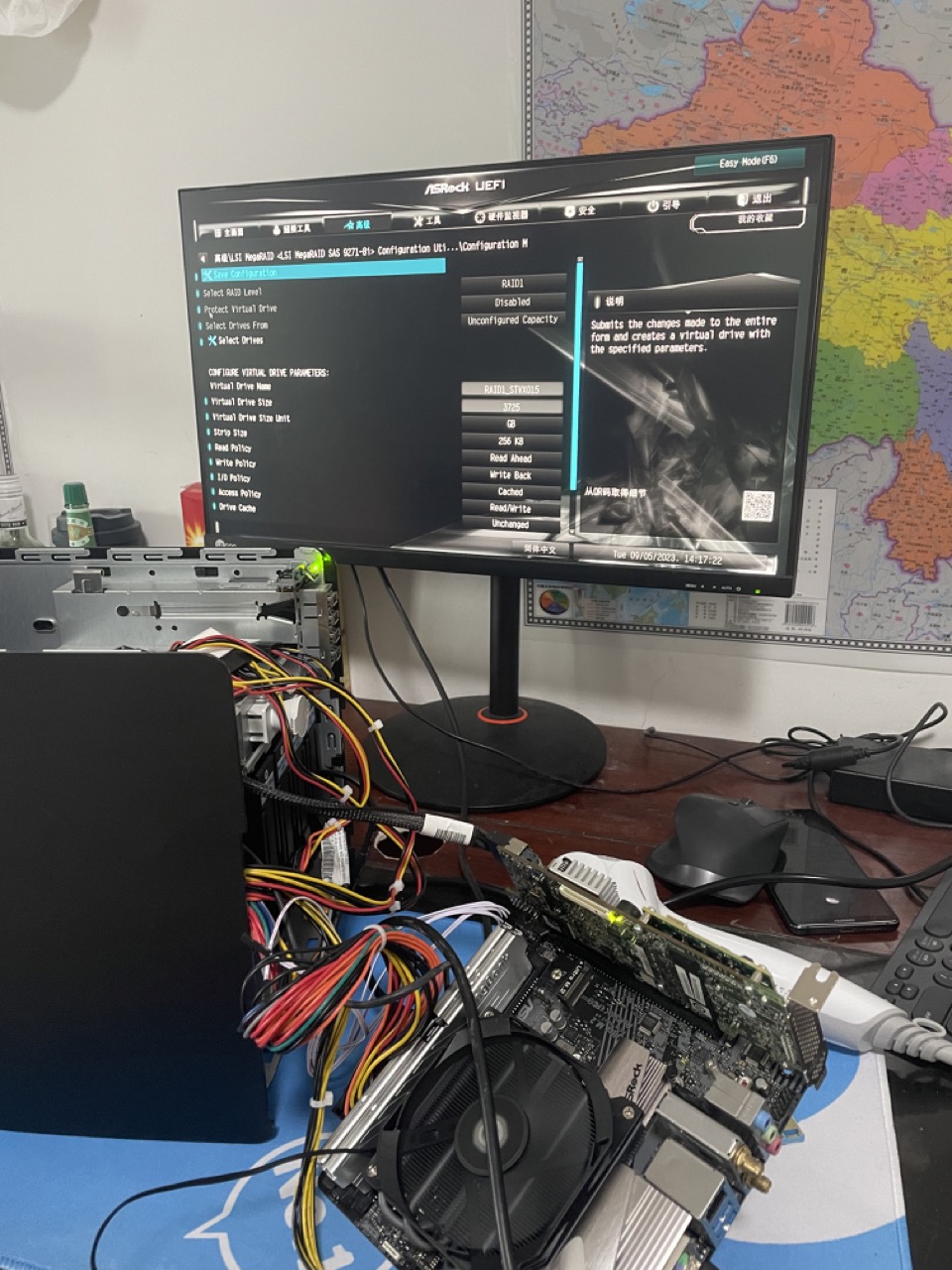
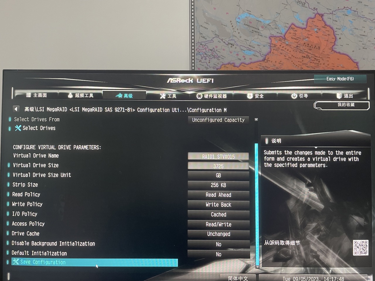
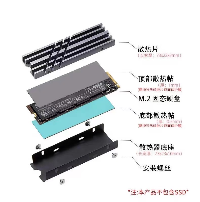
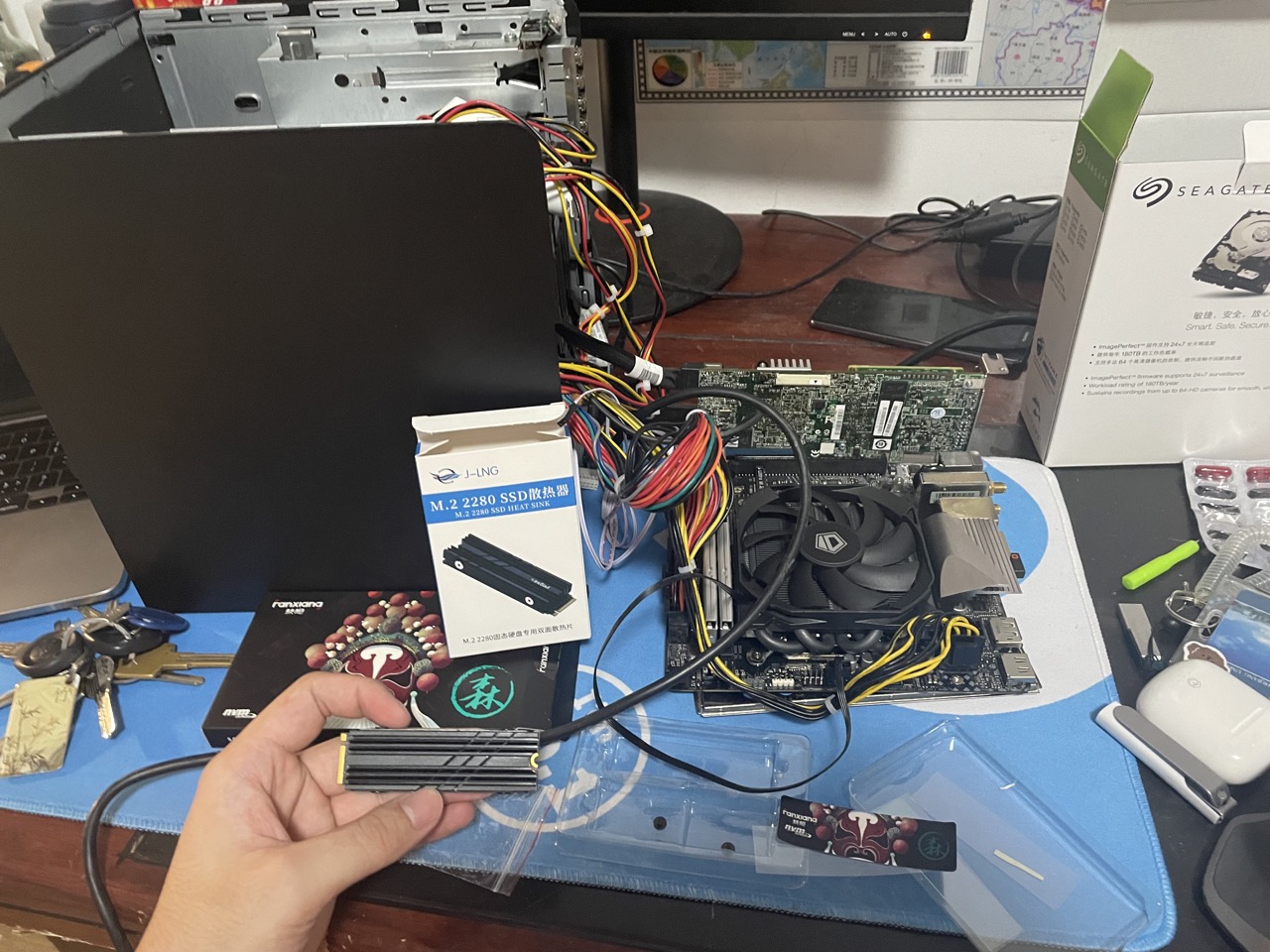

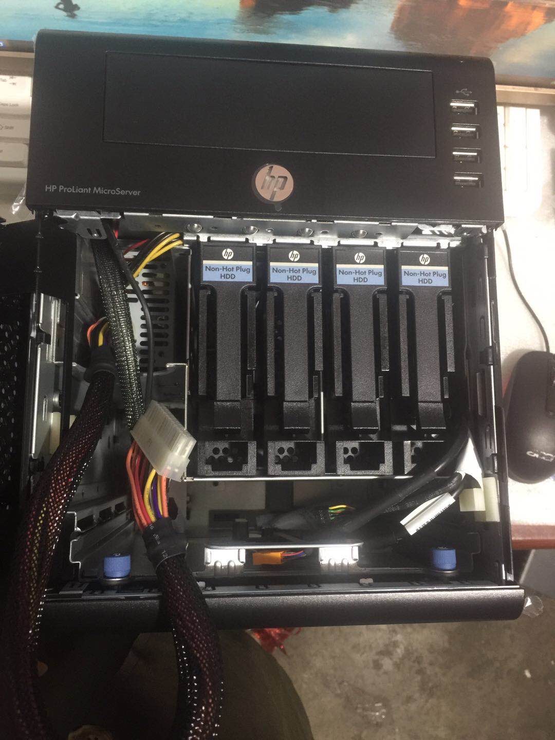


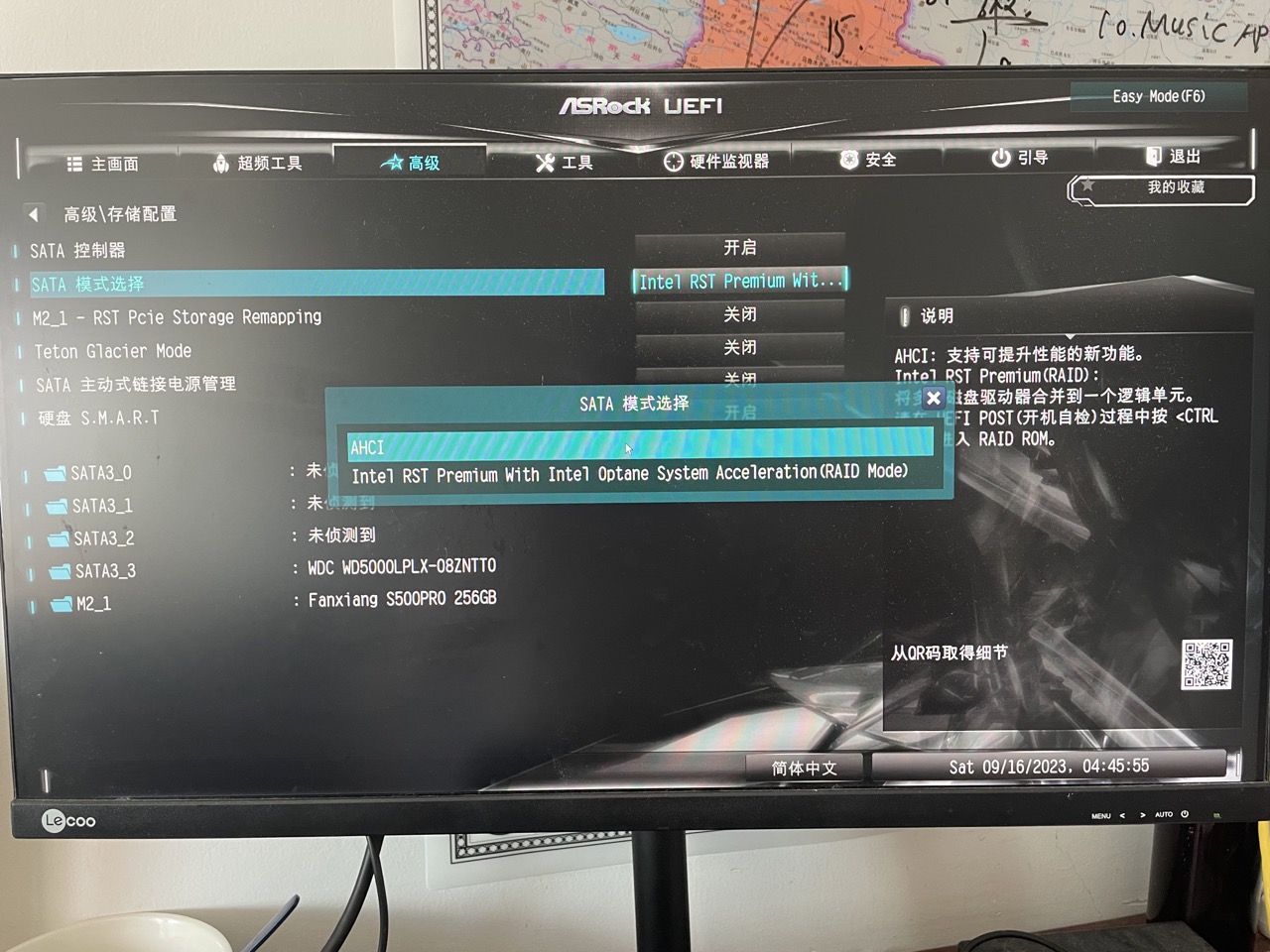


 </img>
 </img>
 </img>
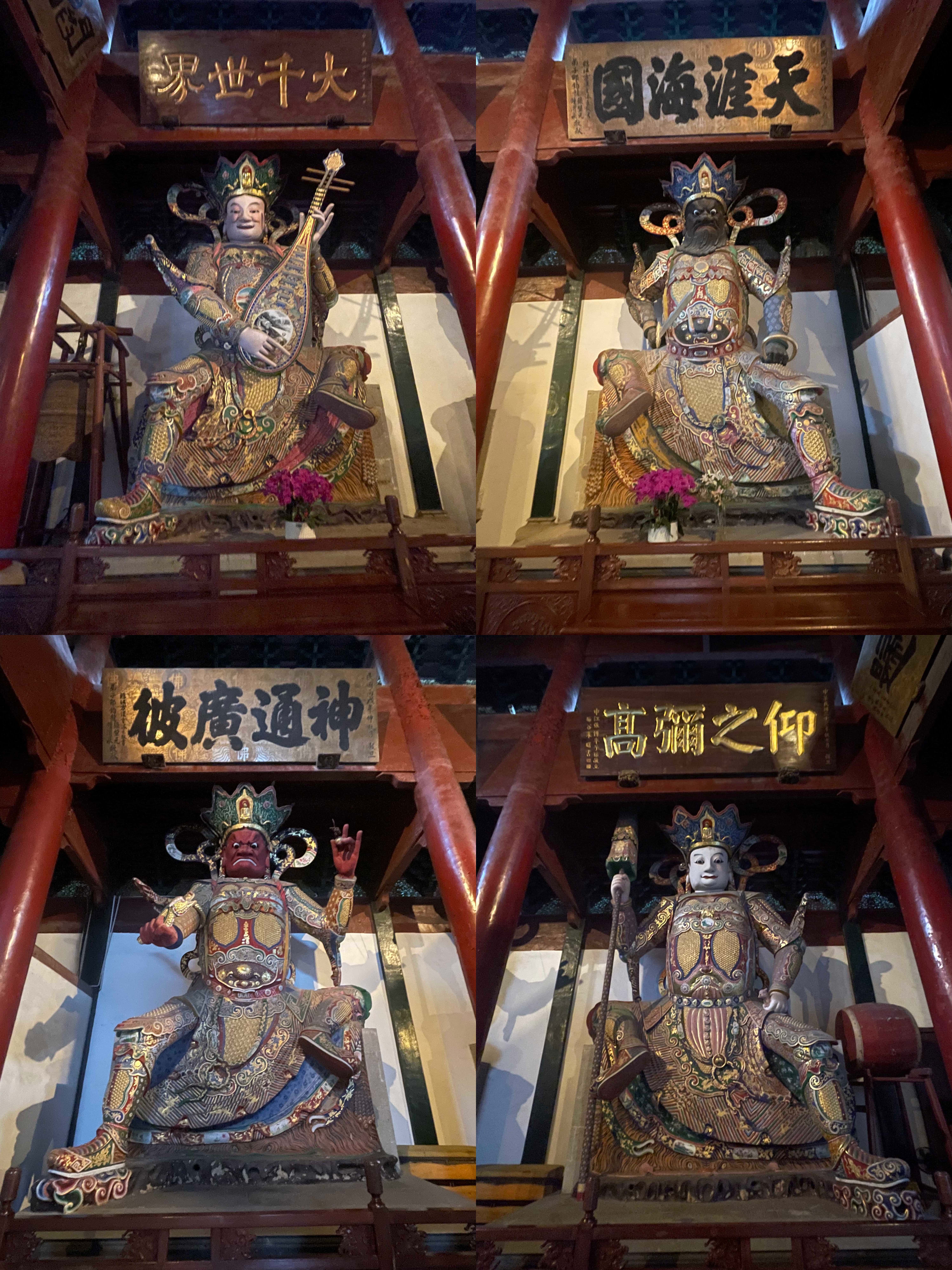
 </img>
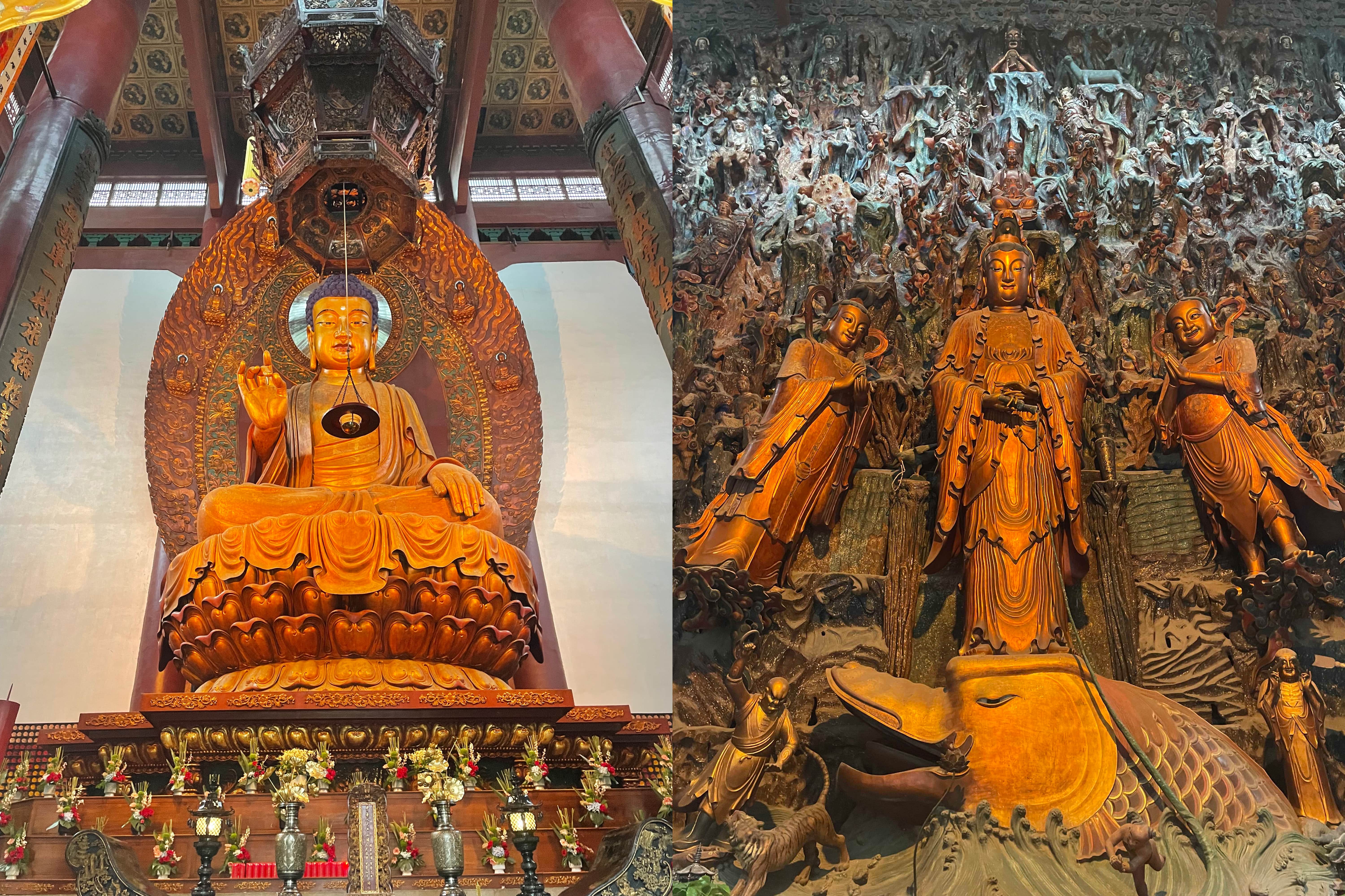
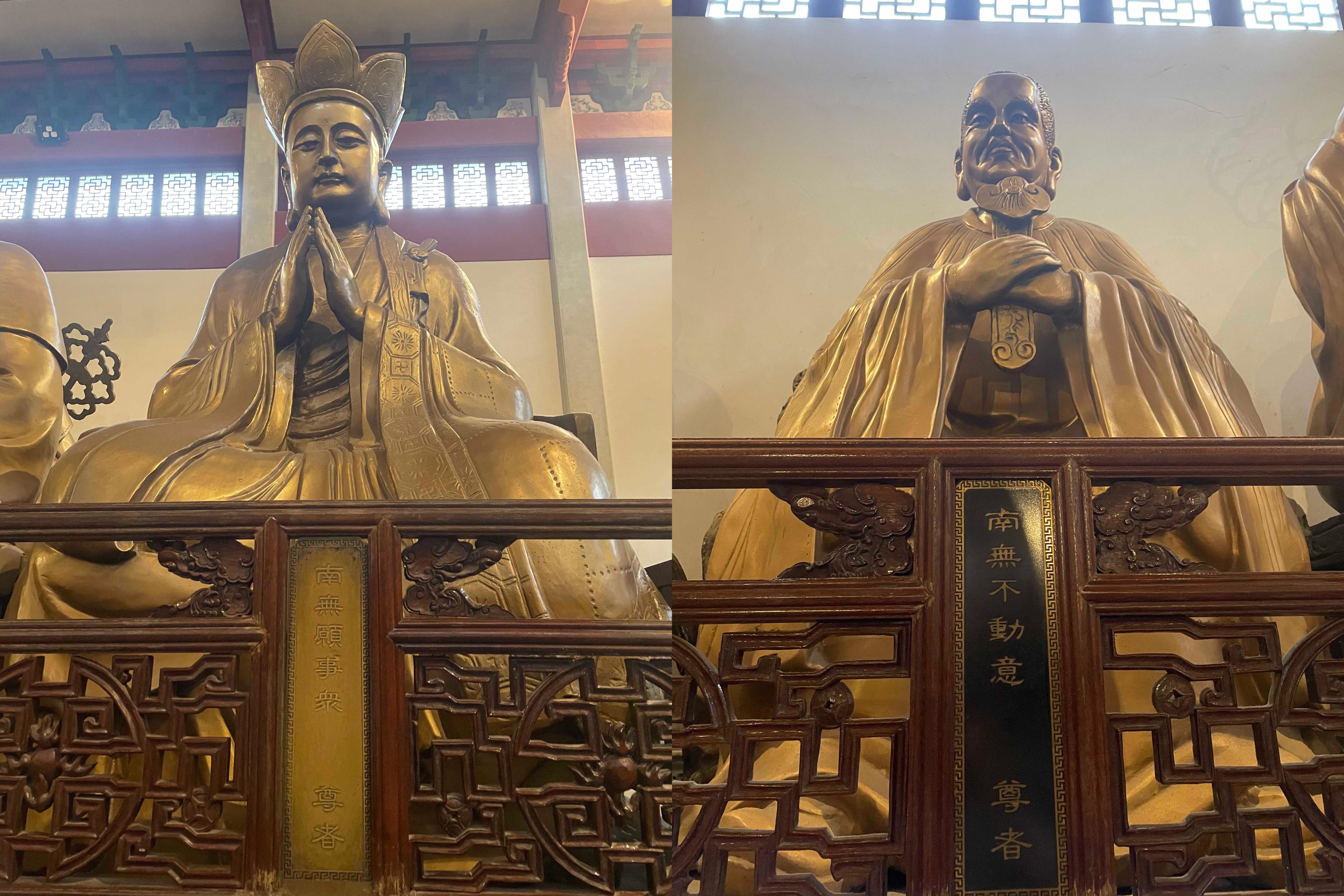 </img>
 </img>
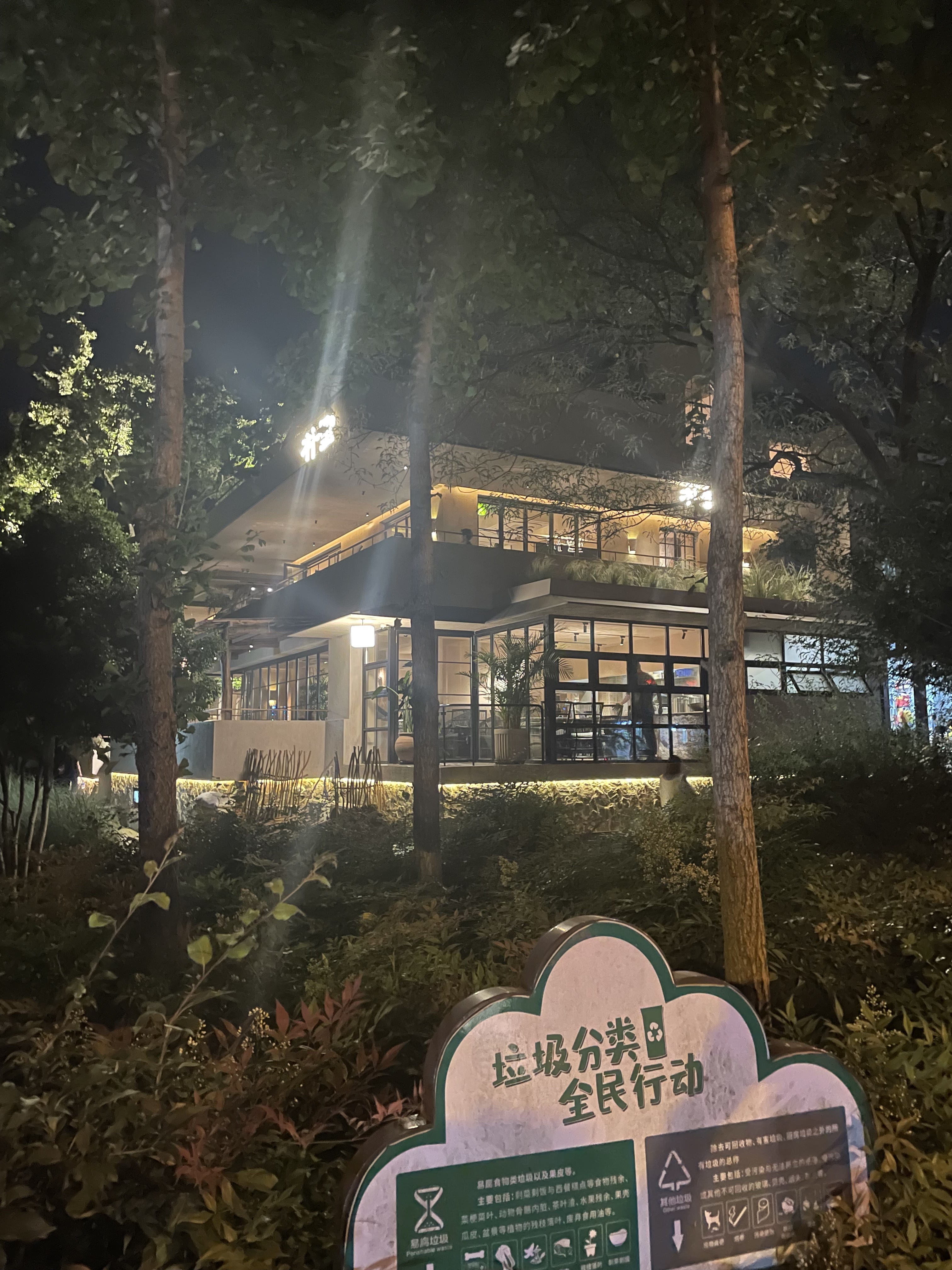 </img>
 </img>
 </img>

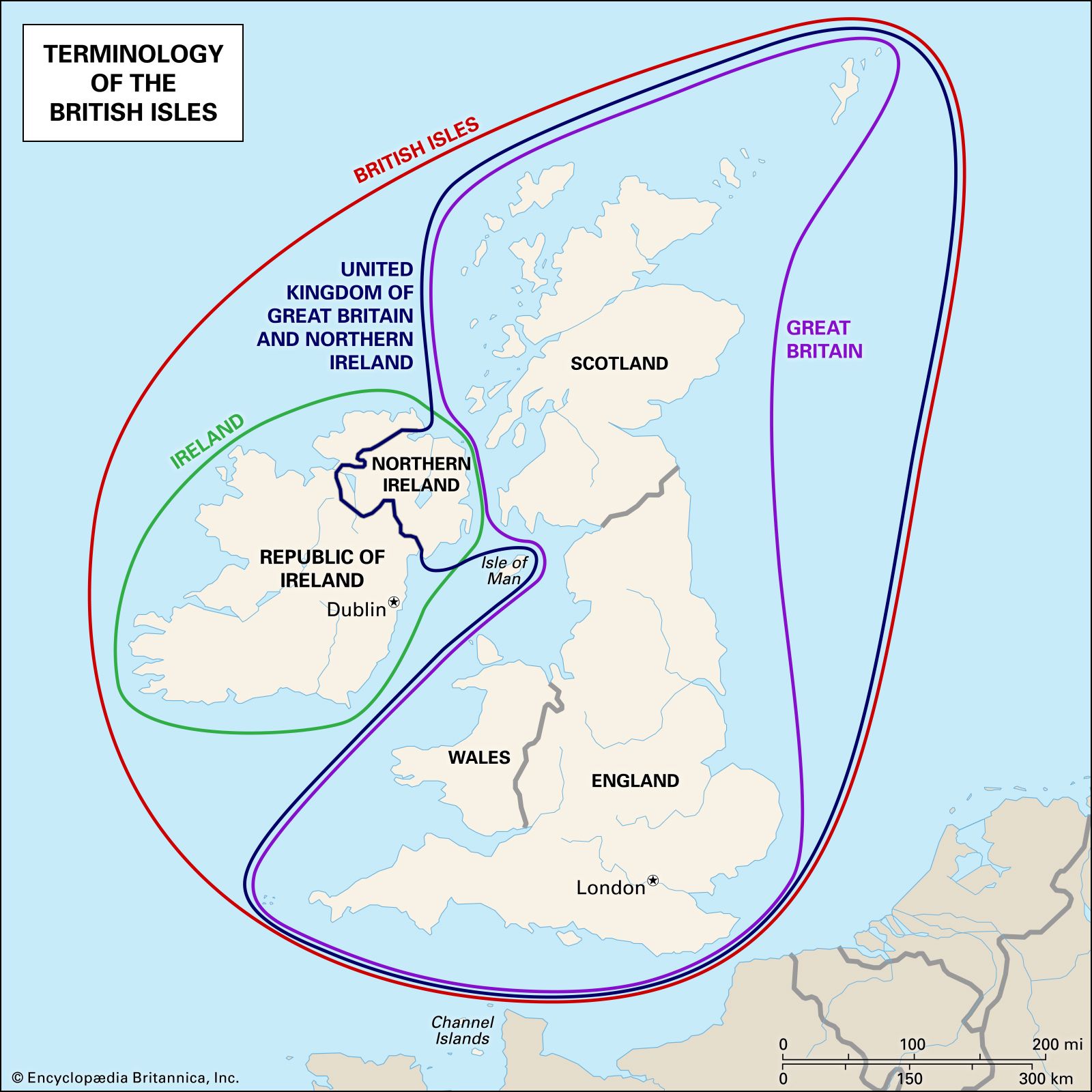 Terminology-British-Isles-United-Kingdom-Ireland-Great
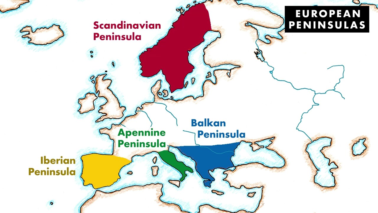 European Peninsulas.
 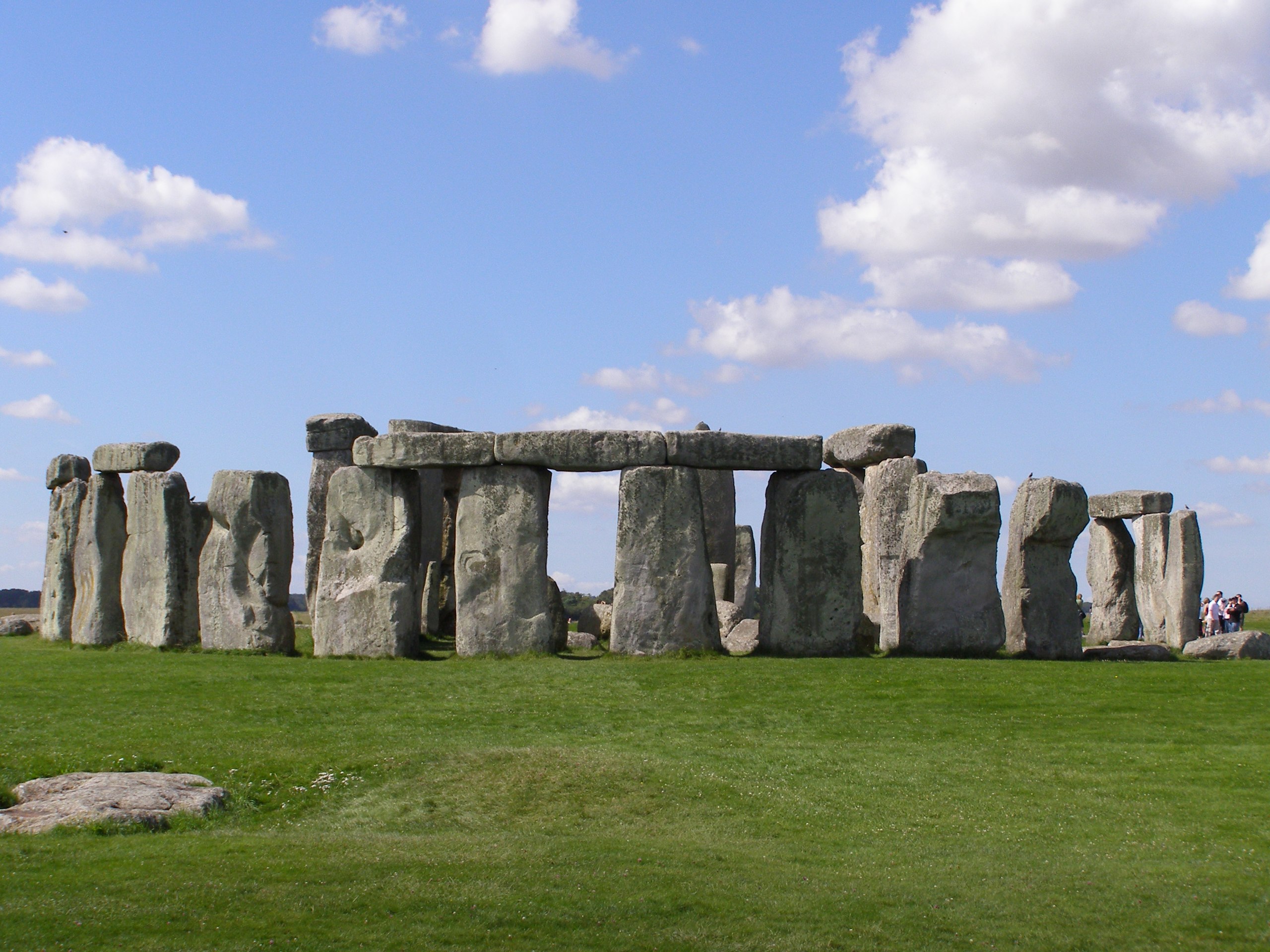 Stone Henge
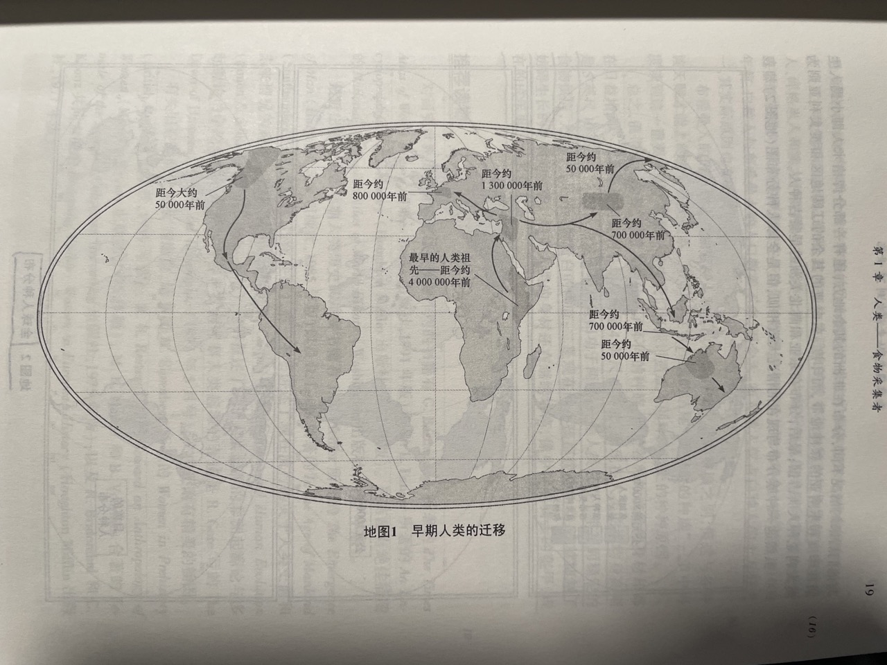 早期人类迁移
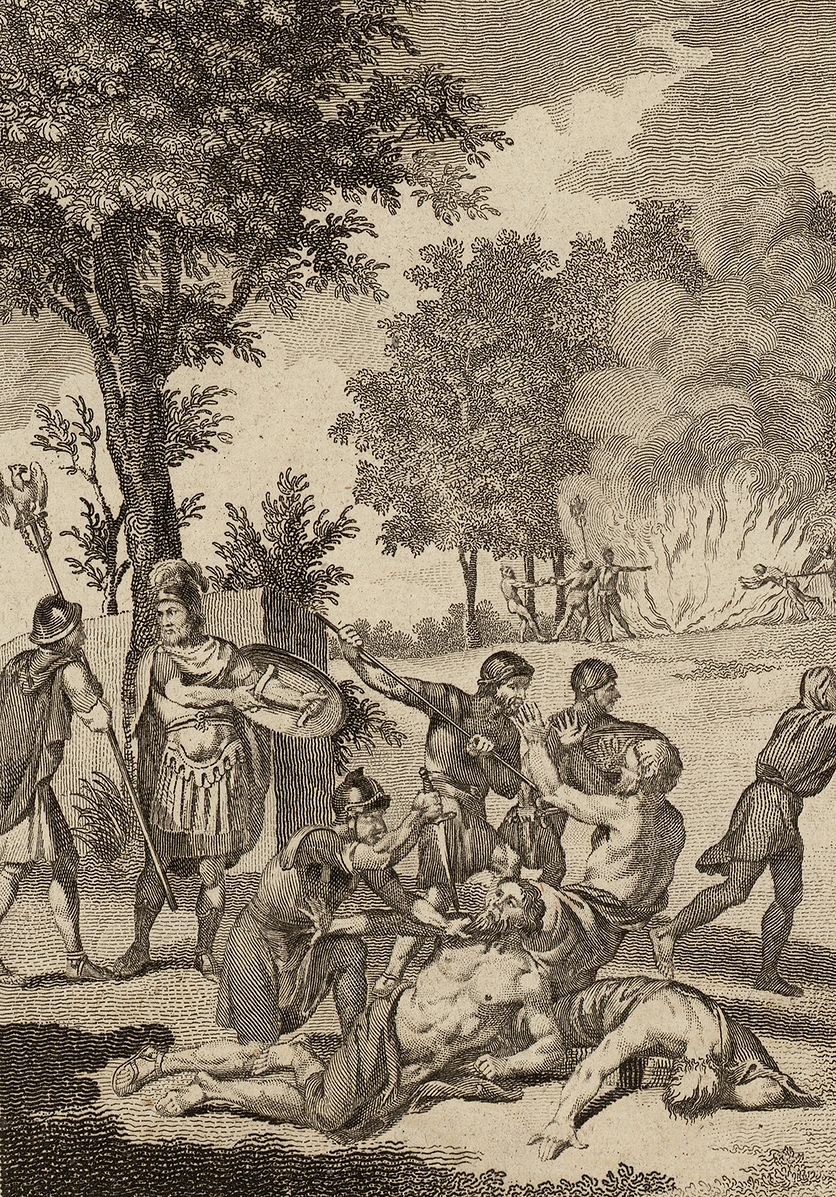 Romans murdering Druids and burning their groves cropped. Most written records are from Tacitus.
.svg.png) Province of Britain in the Roman Empire in 125 AD
Province of Britain in the Roman Empire in 125 AD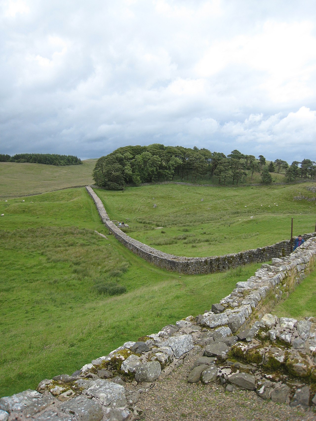
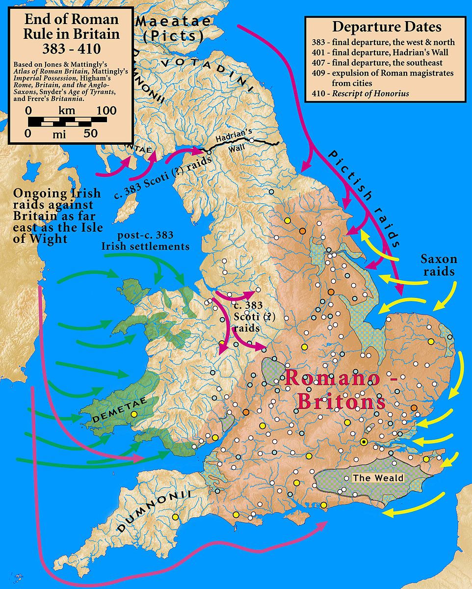
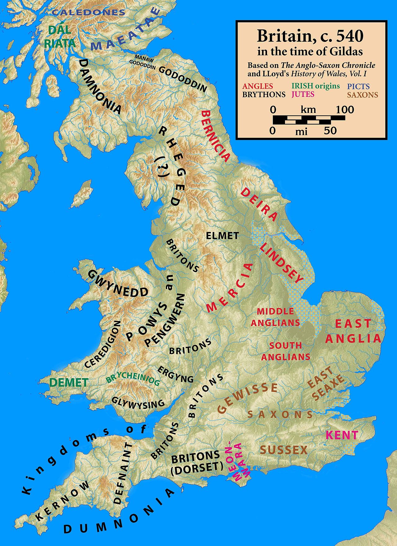
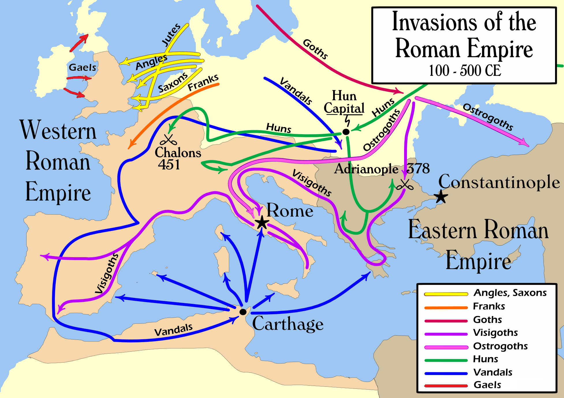
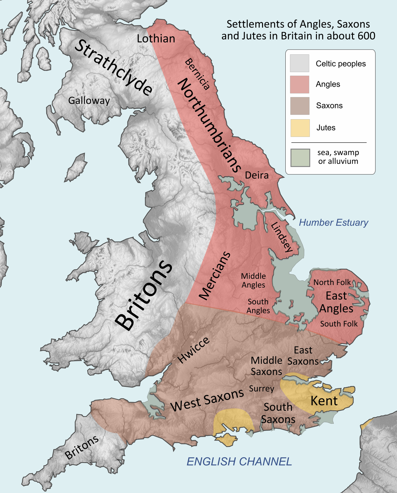 after settlement
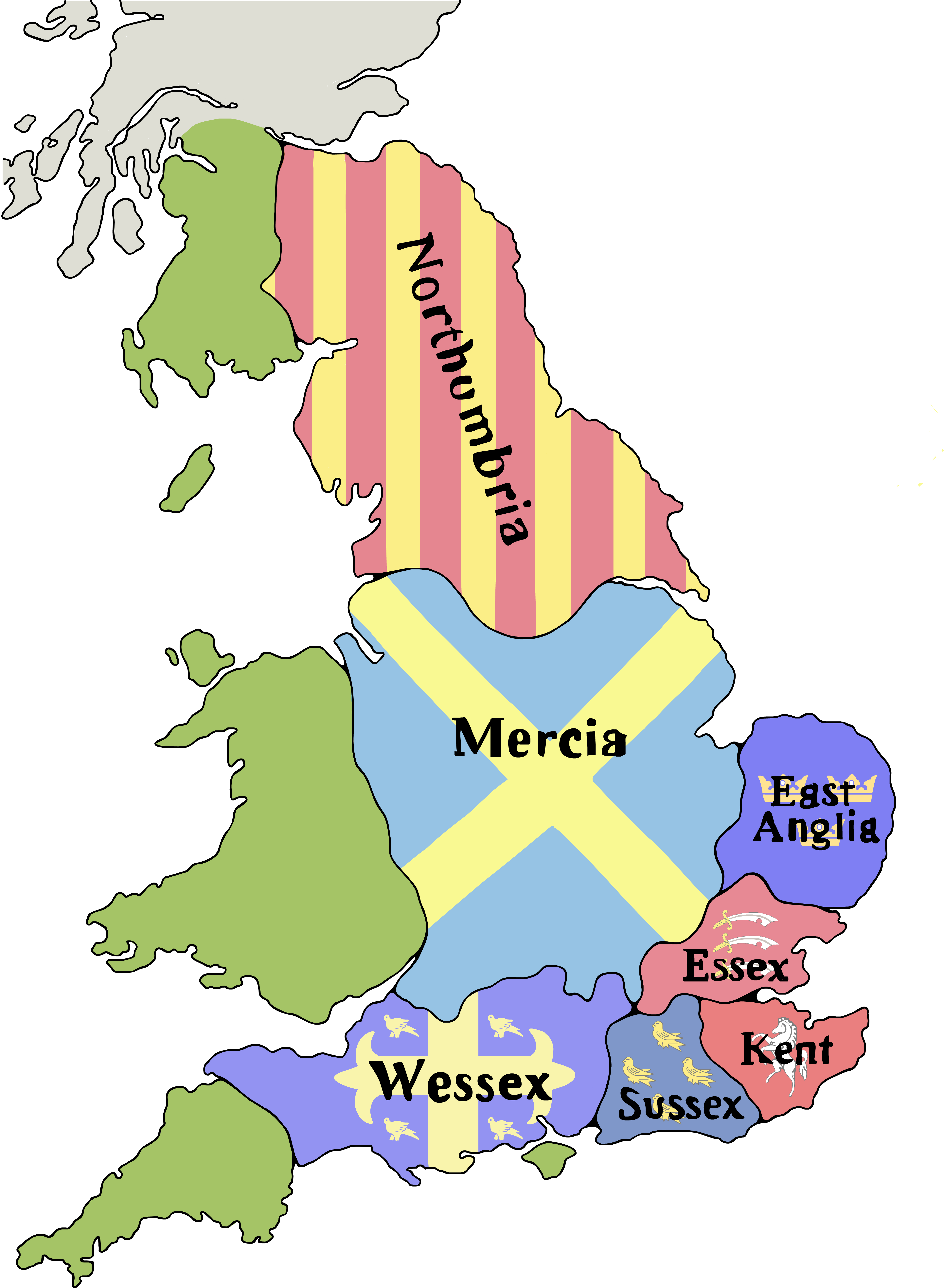
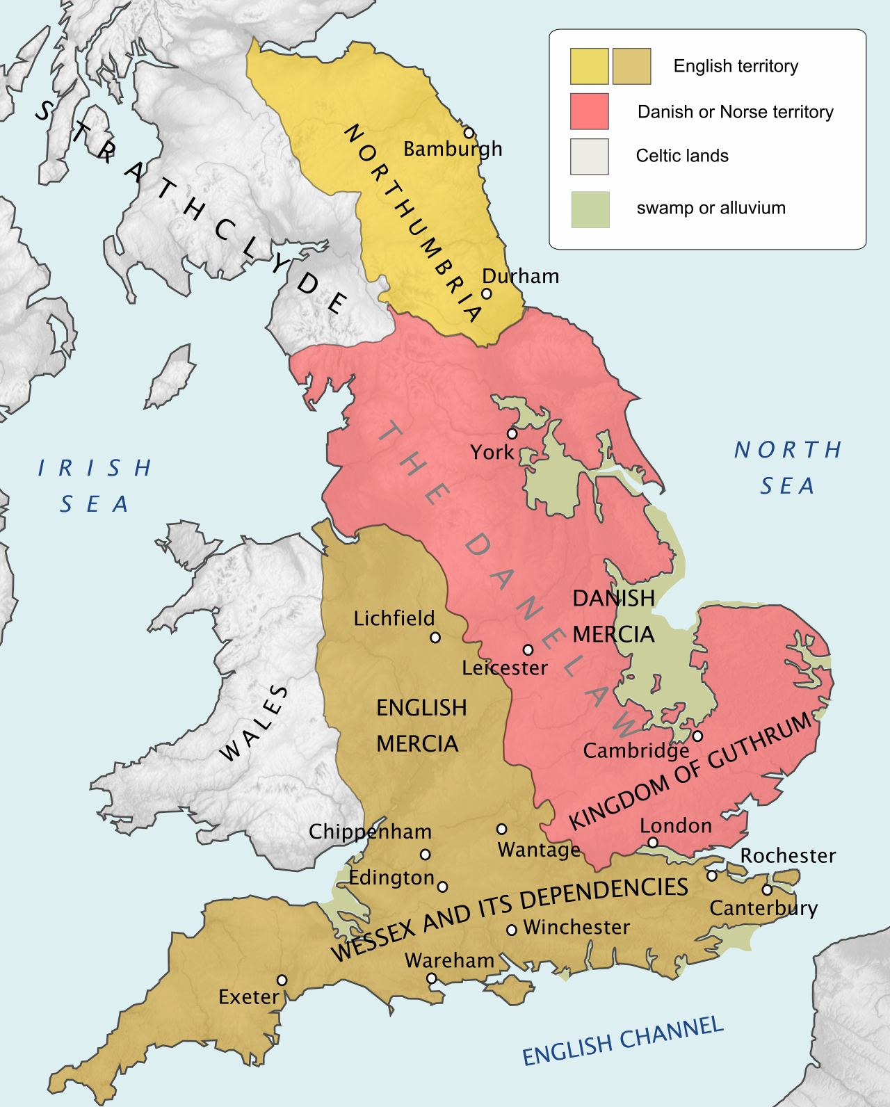
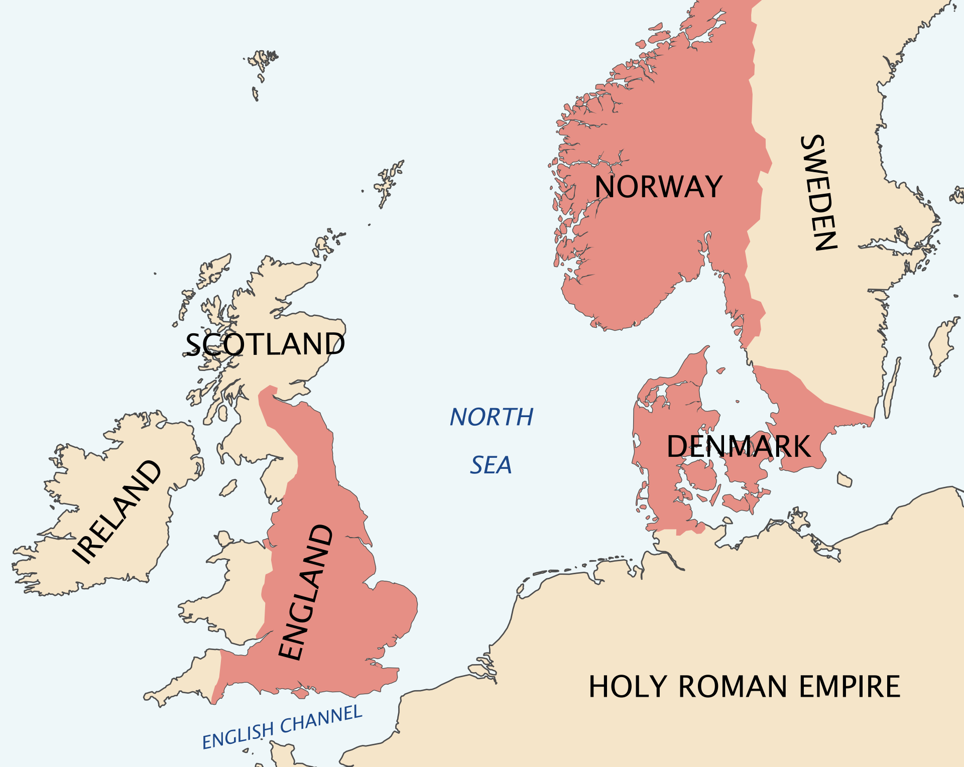
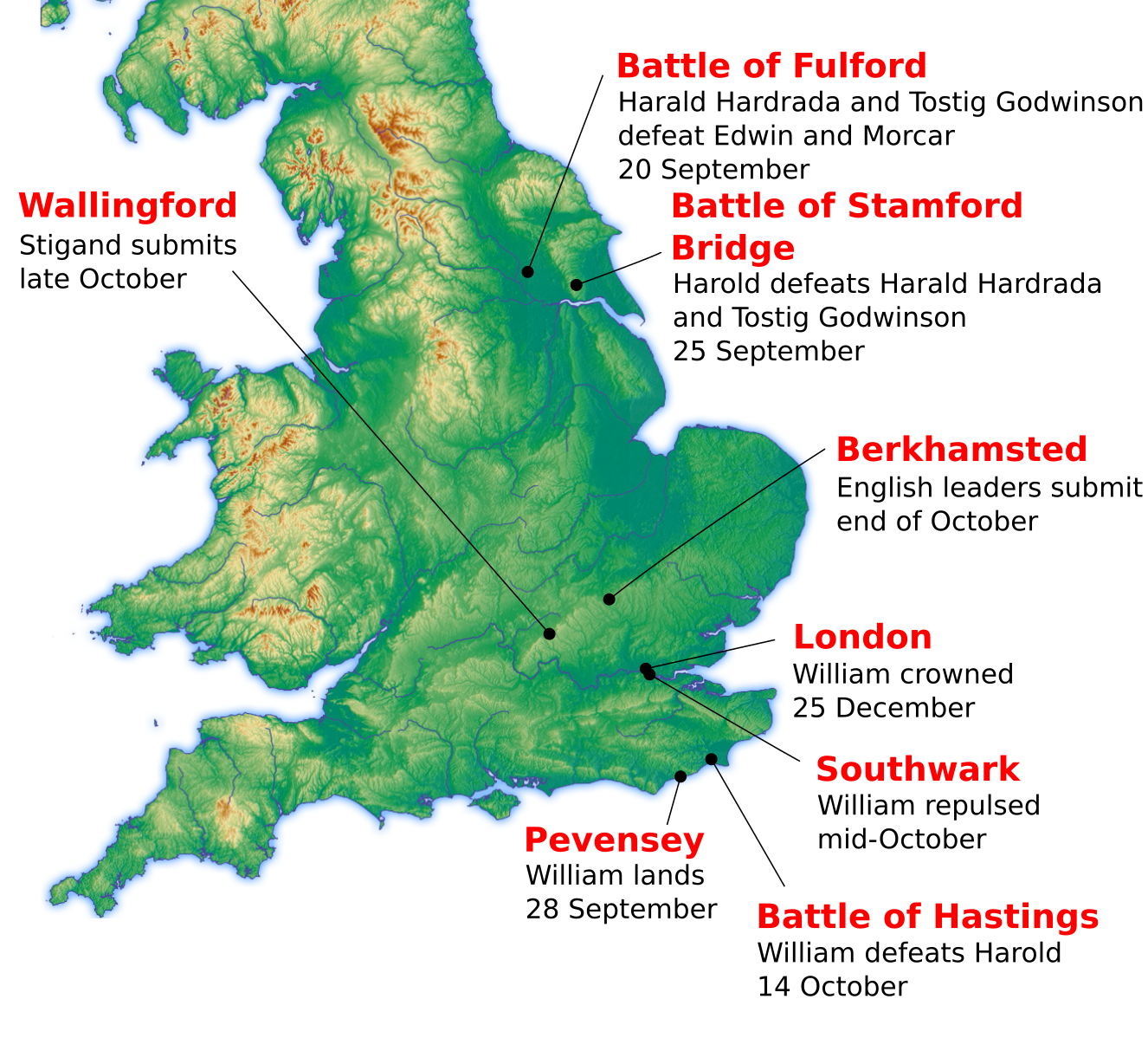
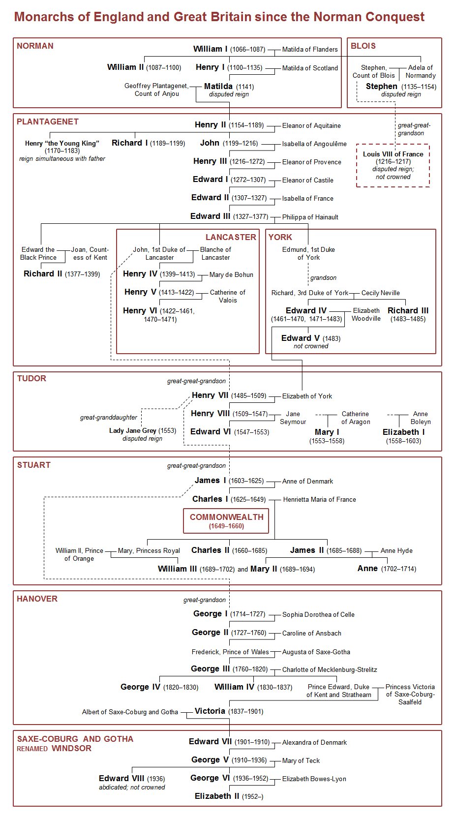
 Statue of Robin Hood near Nottingham Castle by James Woodford, 1951
 Acral gangrene due to plague
  Pieter Bruegel's The Triumph of Death reflects the social upheaval and terror that followed the plague, which devastated medieval Europe.
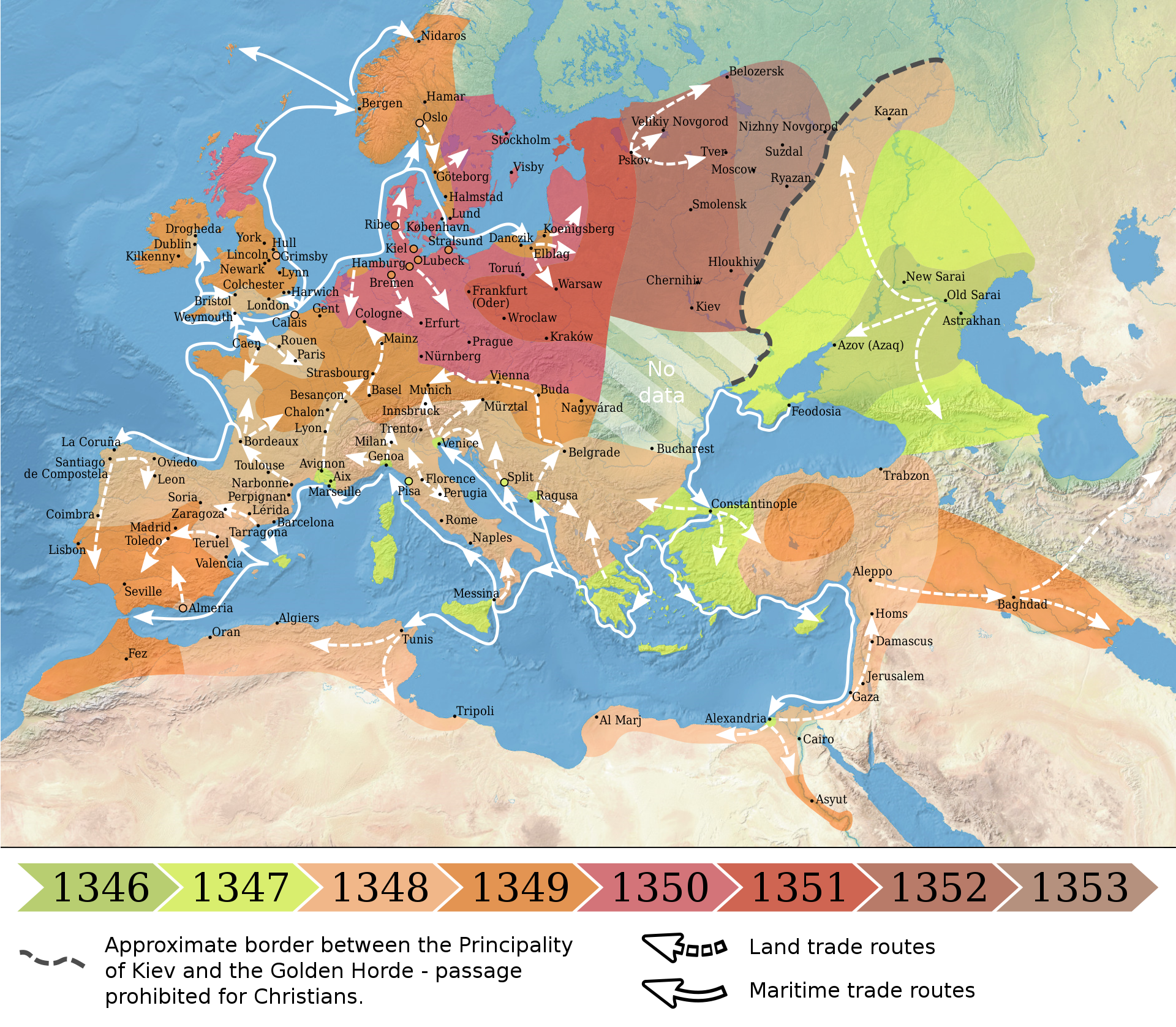
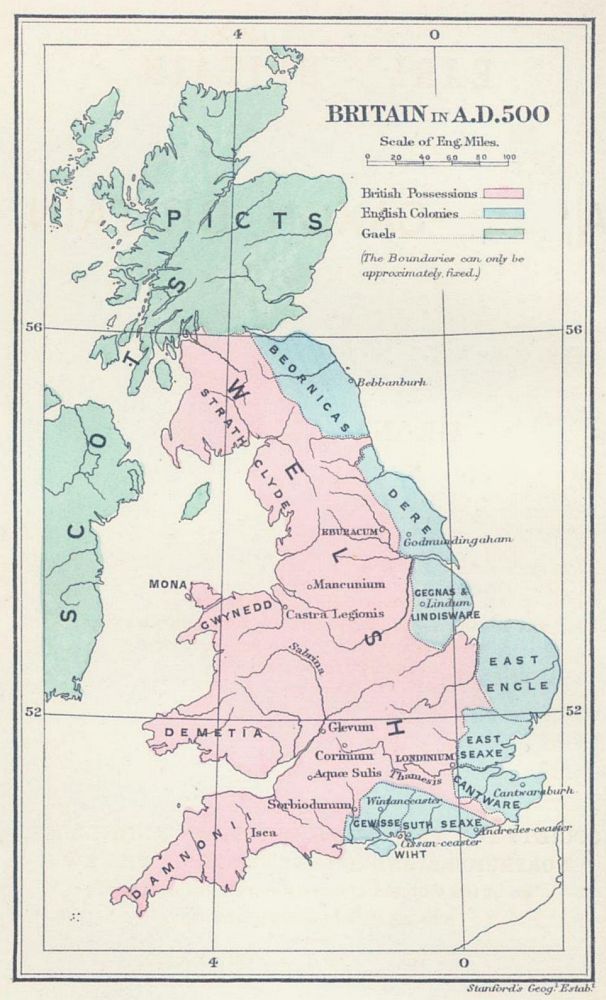

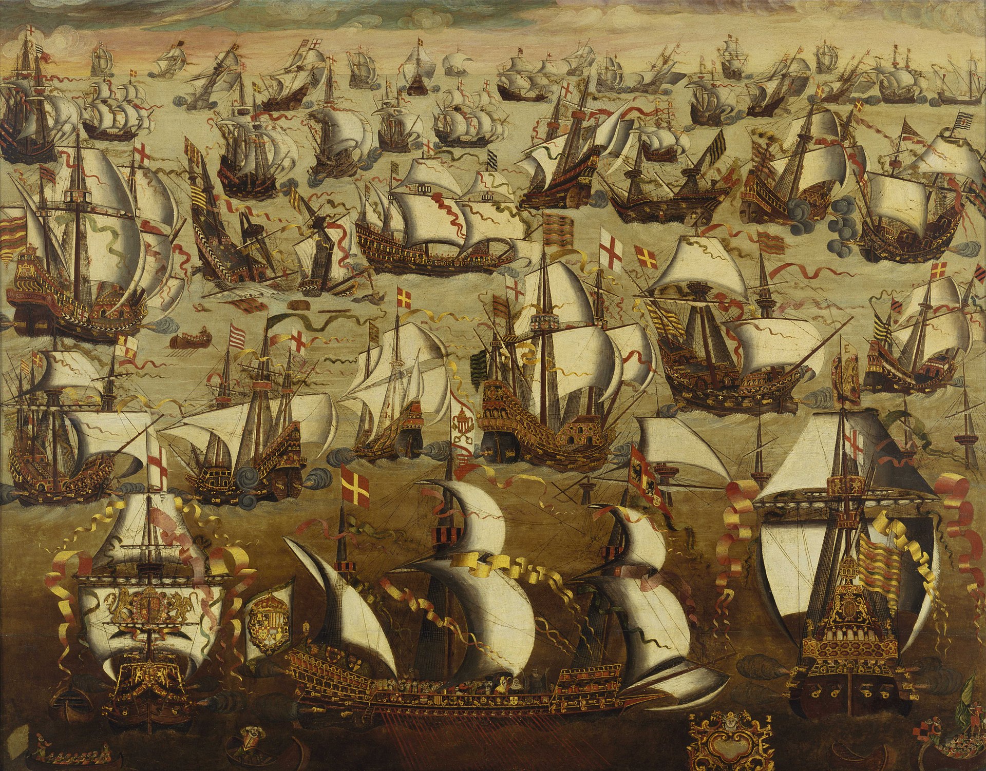 The Spanish Armada fighting the English navy at the Battle of Gravelines in 1588.
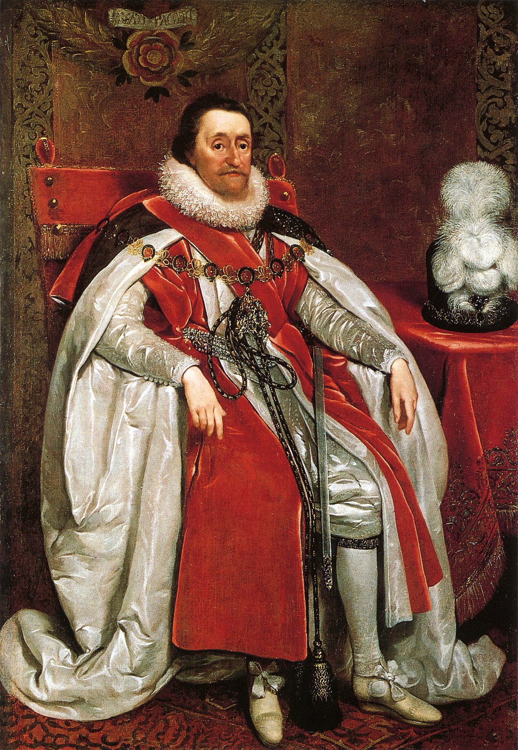 King James VI and I by Mijtens (1621)
_(2022).svg.png)
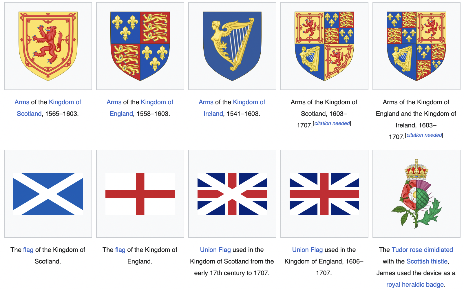
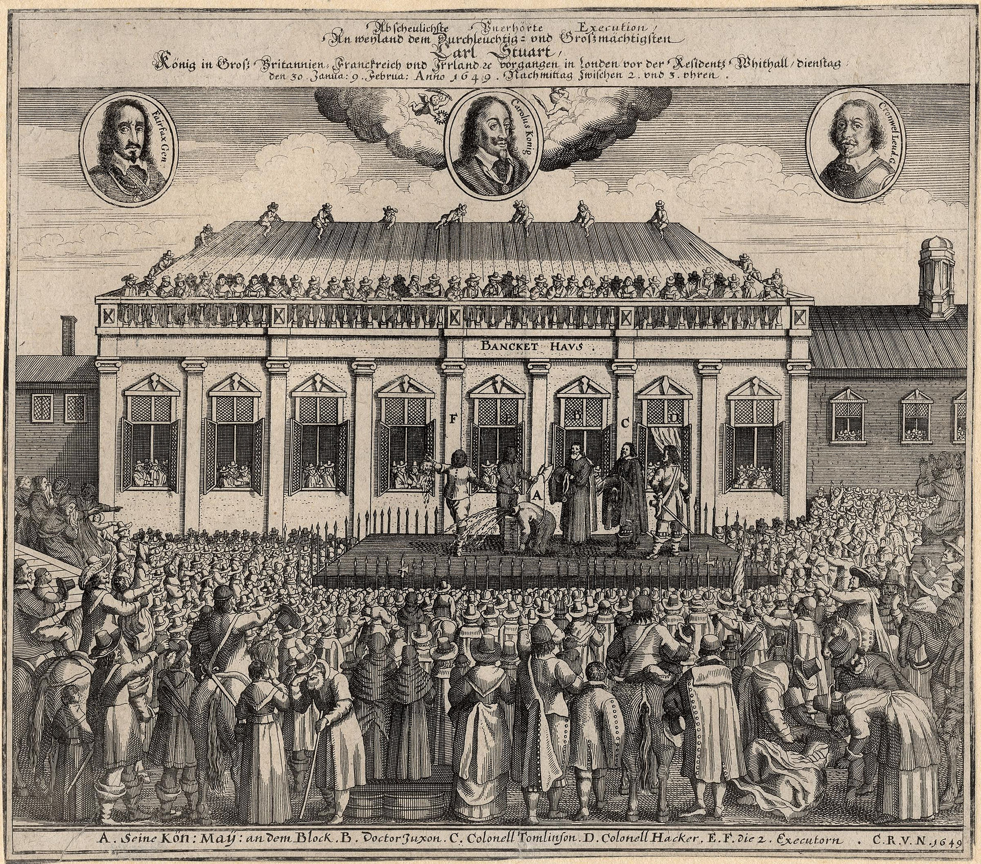
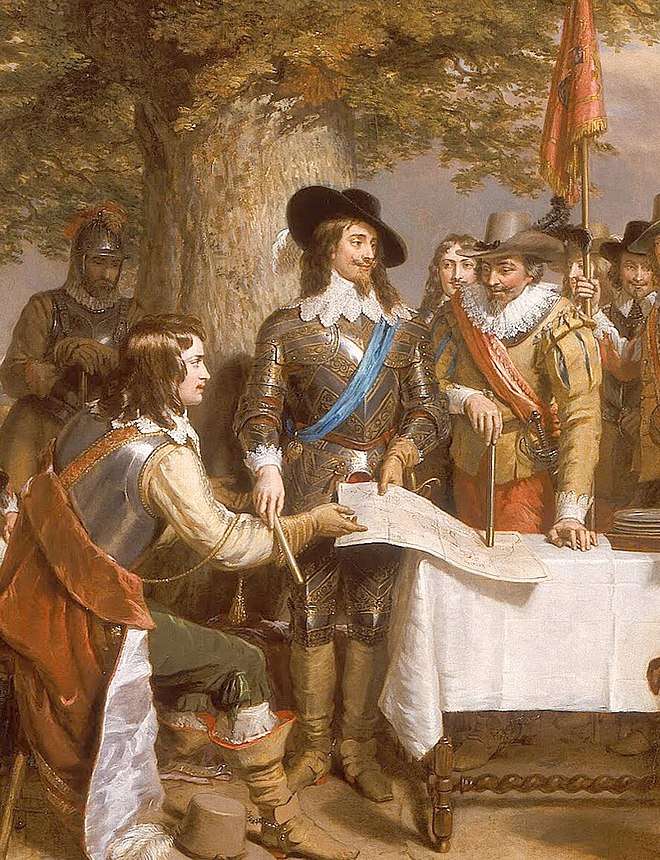 King Charles I, in blue sash, holding a council of war before the Battle of Edgehill in 1642; the cavalry commander Prince Rupert is seated left.
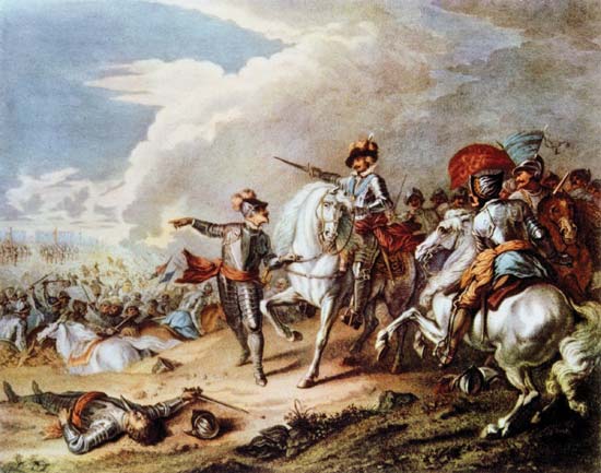 The Battle of Naseby, 14 June 1645; Parliamentarian victory marked the decisive turning point in the English Civil War.
.svg.png) Flag of Great Britain (1707–1801)
Flag of Great Britain (1707–1801)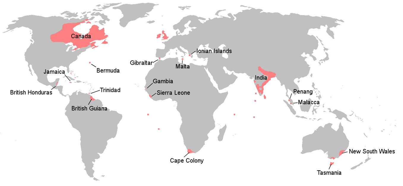 The British Empire at the end of the Napoleonic Wars in 1815
 Flag of the United Kingdom (1801–present)
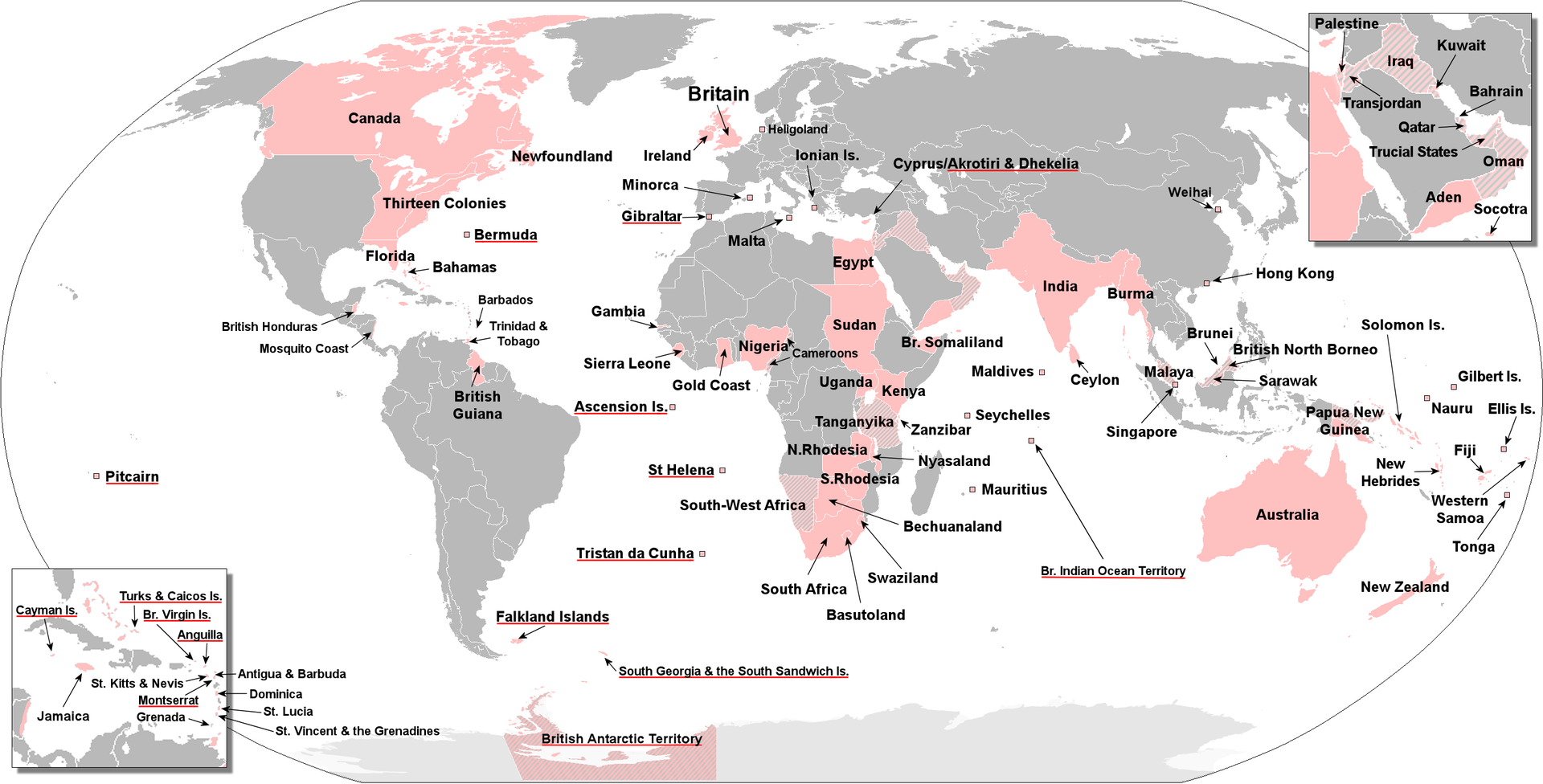 The British Empire at its largest?
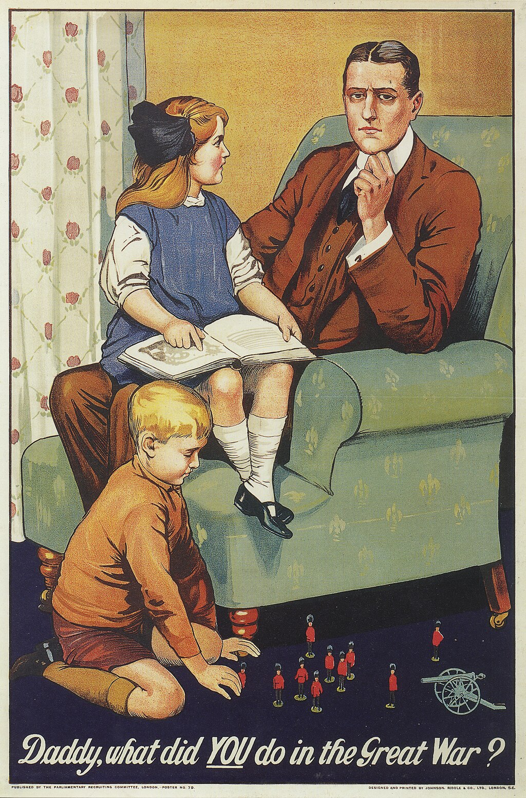 First World War recruiting poster, playing on the guilt of those who did not volunteer
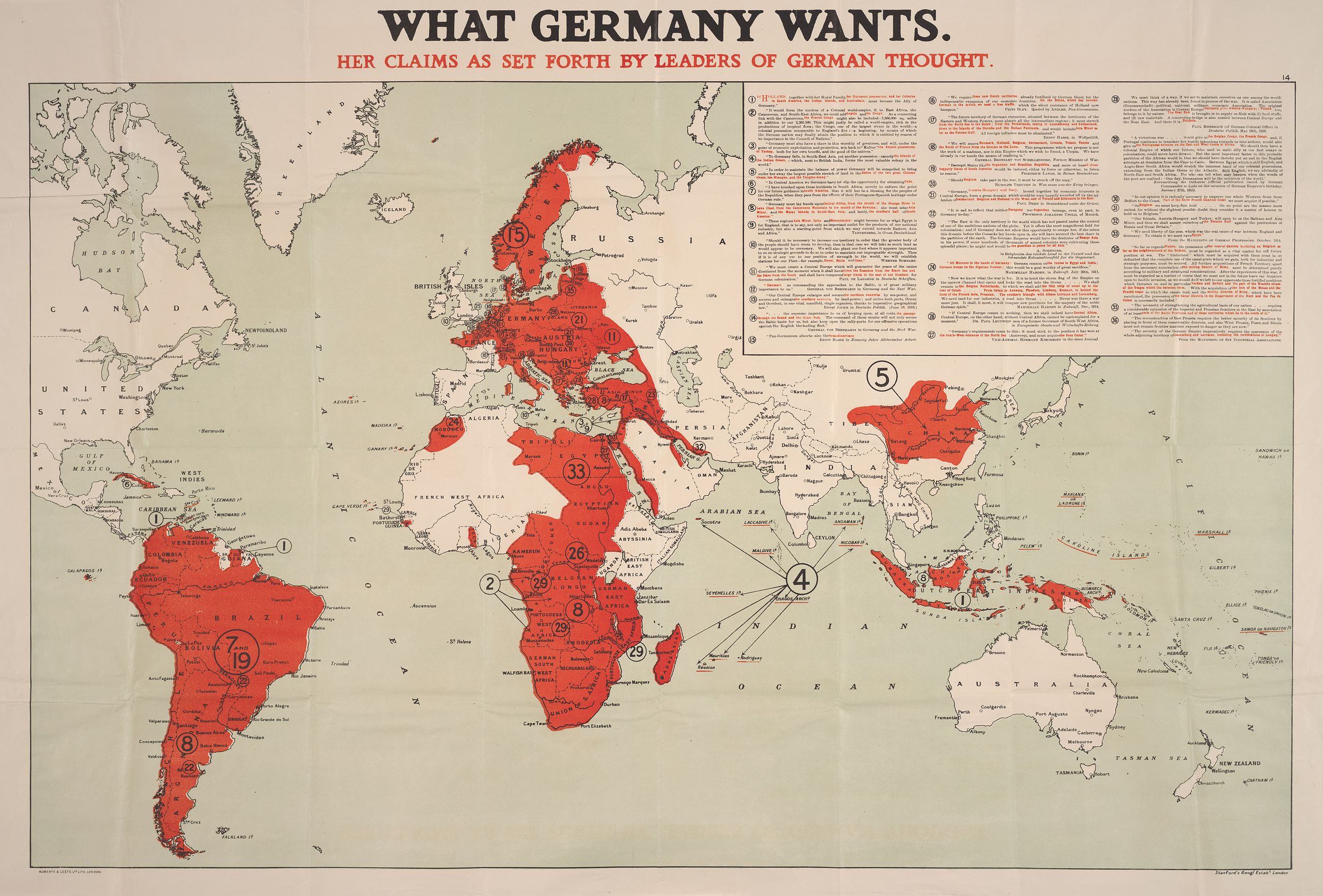 A world map showing territory that "Germany Wants" by Edward Stanford. 1917. Close reading of the quoted material shows that the map is misleading: it implies that Germany plans to annex all the territory in red, but this is only the case for a small fraction of it.
_map_-_winning_party_vote_share_by_constituency.svg.png) Result of the 1918 UK general election in Ireland
Result of the 1918 UK general election in Ireland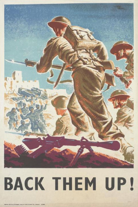
 </img>
.svg.png)
 </img>
</img>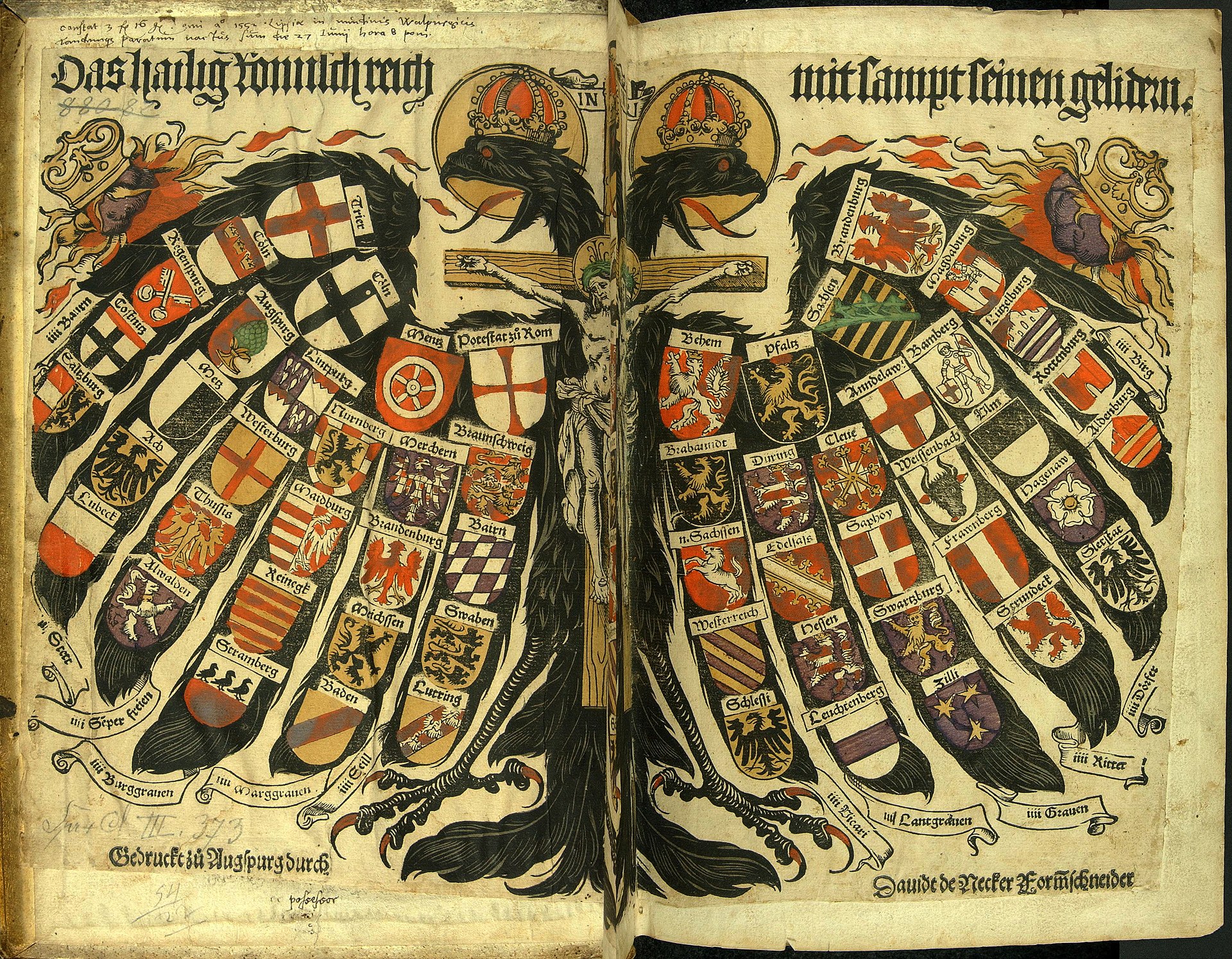
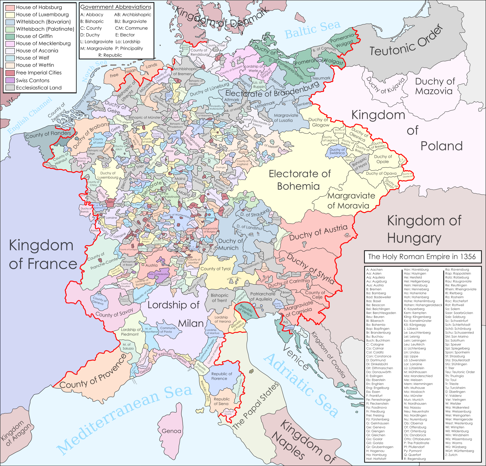 </img>
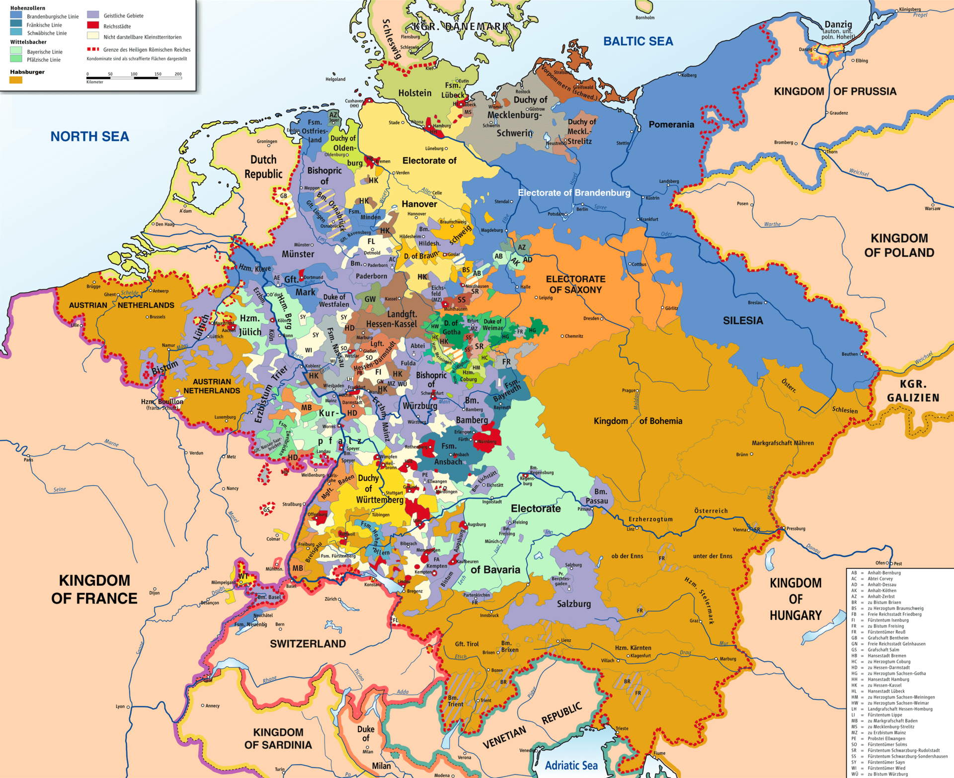
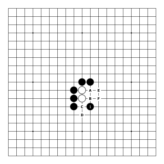


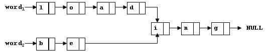
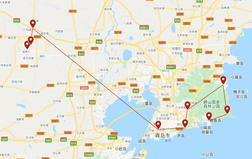
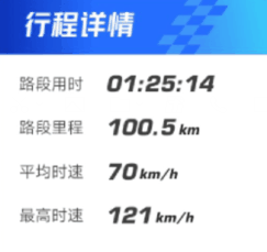

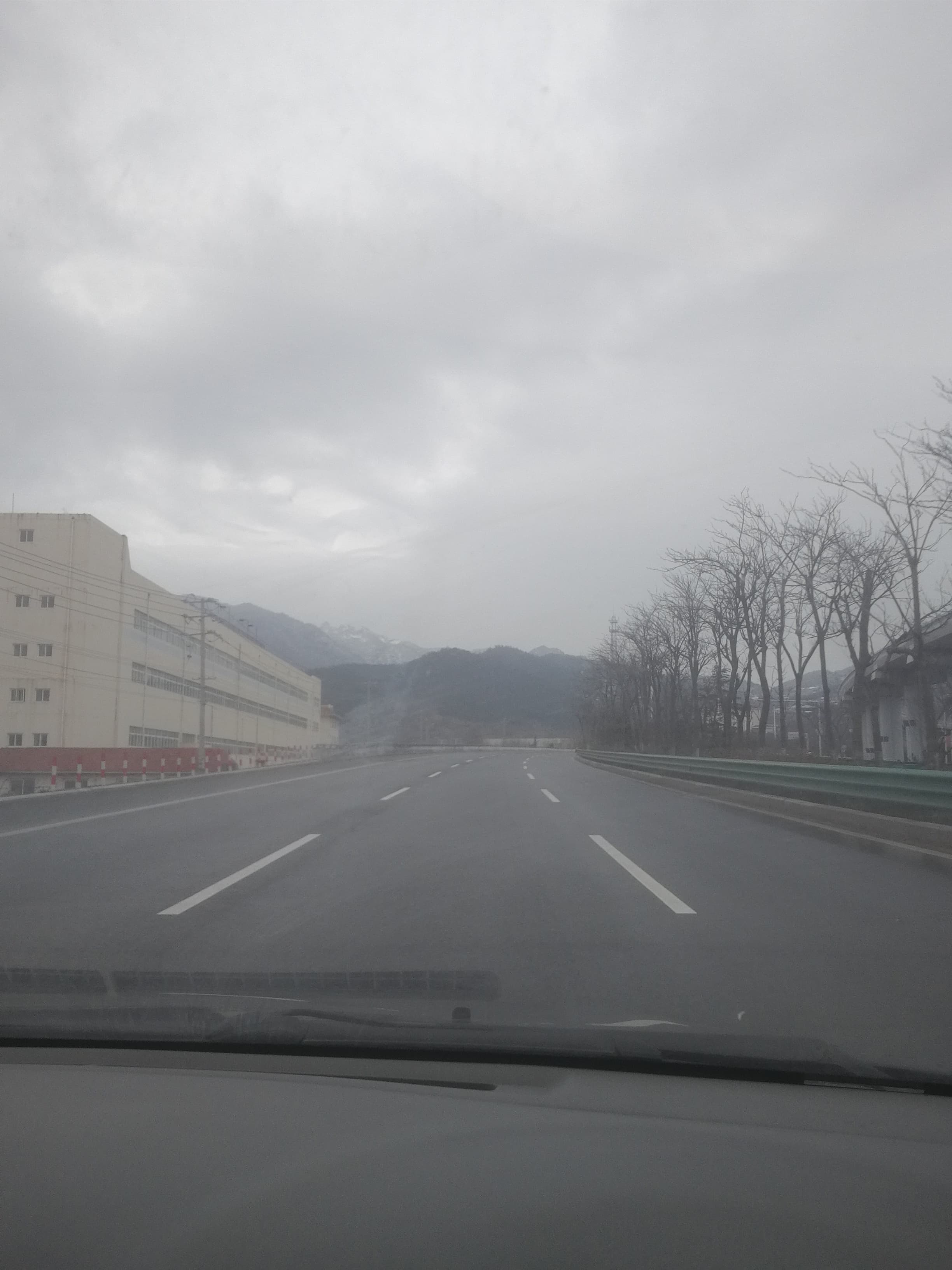


 |
|  |
|